Step 1 of 8
Set Up a Small, Checkable Table
Set up a small spreadsheet table, distinguish its inputs from its output locations, and establish a manual check for the first week before asking an AI for a formula.

Learning path · Level 5 · Tutorial 2
Use a small table entered in your own spreadsheet to request and inspect AI-suggested formulas. Check results against simple calculations and assess whether an accompanying trend explanation matches the spreadsheet data.

 Set Up a Small, Checkable Table
Set up a small spreadsheet table, distinguish its inputs from its output locations, and establish a manual check for the first week before asking an AI for a formula. 2 min
 Request a Formula with Exact Context
Create a precise AI request for the practice spreadsheet so that suggested formulas can be checked against known values. 3 min
 Read the Formula Before Using It
Inspect arithmetic and SUM formulas before using them, including the references, operations, range endpoints, and locale-sensitive syntax. 3 min
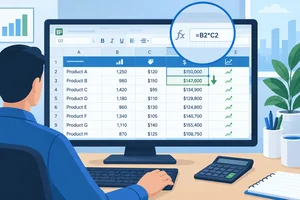 Test One Row, Then Check the Copy
Verify the first weekly revenue formula, then confirm that filling it down preserves the intended row-by-row logic. 3 min
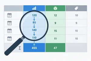 Check What the Total Includes
Validate spreadsheet totals by checking range coverage, selected columns, and an independent addition. 2 min
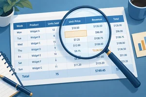 Find Missing Values and Text Numbers
Diagnose blank inputs and numeric-looking text entries without confusing them with an incorrect SUM range. 3 min
 Check the Trend Explanation
Check an AI-generated trend explanation against comparable periods, consistent units, and the verified values in the Practice worksheet. 3 min
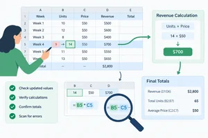 Complete a Formula and Explanation Check
Update a small spreadsheet table, verify formula suggestions against independent checks, and write an evidence-supported trend explanation. 4 min
Step 1 of 8
Set up a small spreadsheet table, distinguish its inputs from its output locations, and establish a manual check for the first week before asking an AI for a formula.
Create or rename a worksheet to Practice. You will enter and check everything in your own spreadsheet; an AI assistant cannot see or edit it unless you explicitly share content.
A cell address combines its column letter and row number. For example, B2 is column B, row 2. In this task, columns B and C hold source inputs, while column D is reserved for weekly revenue outputs.
Each data row is one complete, consecutive seven-day period for the same product. Revenue excludes discounts, taxes, and returns.
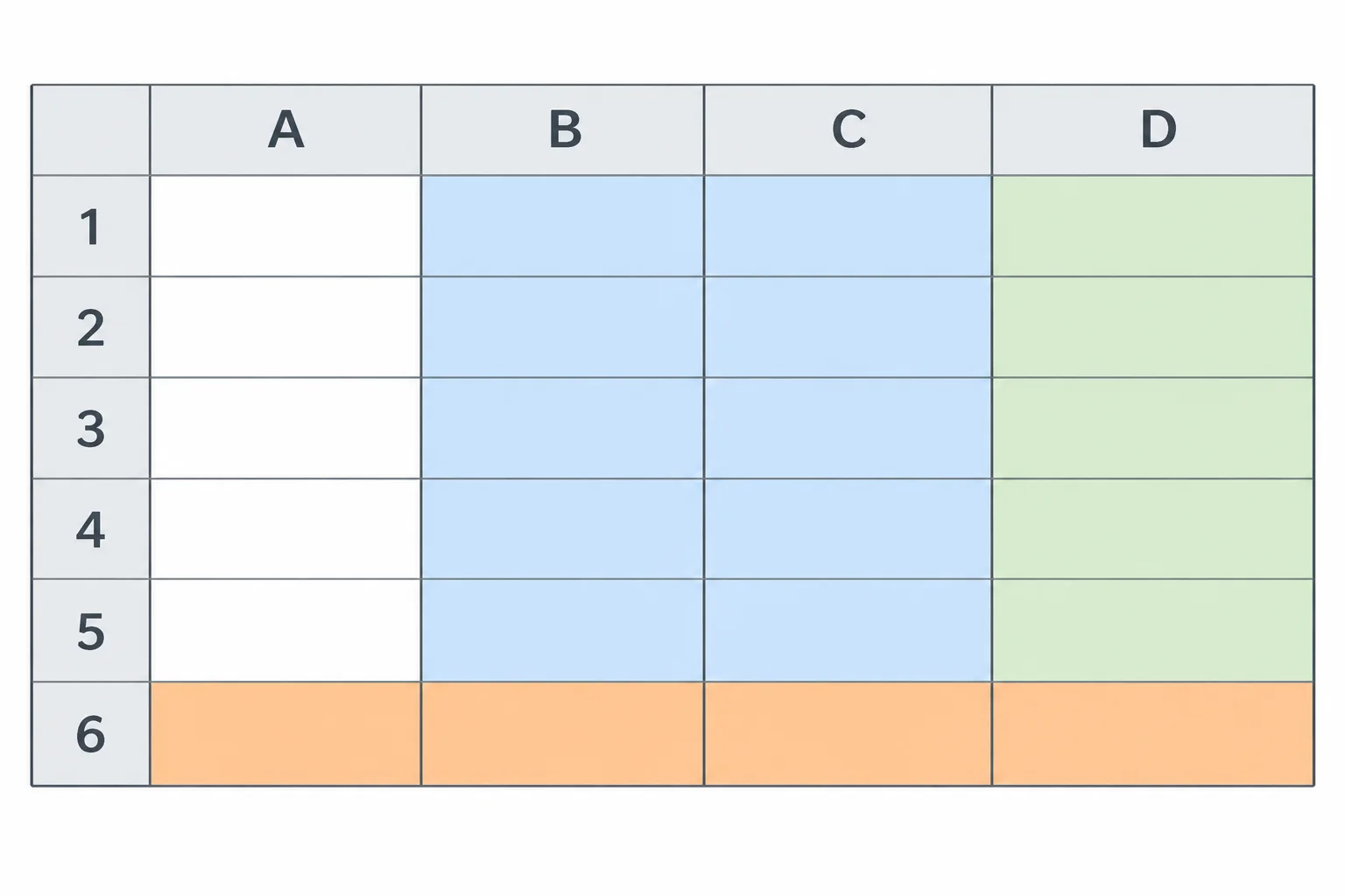
Use the column letters and row numbers to locate a cell precisely. Columns B and C are inputs; D2:D5 will hold weekly revenue outputs later.
Enter the headers and source values below exactly as shown. Enter source values as plain numbers: do not type currency symbols into the cells.
Type Total in A6. Leave D2:D5 empty for now: they are reserved for weekly revenue calculations. Also leave B6, C6, and D6 empty for now; the summary outputs will be calculated later.
The data is synthetic and intentionally small, so every later result can be checked independently.
Use this as your entry map for the worksheet named Practice.
| Row | A | B | C | D |
|---|---|---|---|---|
| 1 | Week | Units sold | Unit price (USD) | Revenue (USD) |
| 2 | Week 1 | 10 | 5 | |
| 3 | Week 2 | 12 | 5 | |
| 4 | Week 3 | 8 | 10 | |
| 5 | Week 4 | 10 | 10 | |
| 6 | Total |
Match each cell location to its role in the practice sheet.
Tap an item and then its matching pair.
Without using AI or a spreadsheet formula, use the Week 1 row to write:
This independent check is the result you will use to evaluate a later formula suggestion.
Write at least 35 characters (0/35).
Step 2 of 8
Create a precise AI request for the practice spreadsheet so that suggested formulas can be checked against known values.
An AI assistant cannot see or edit your spreadsheet unless you explicitly provide the information. Treat your request as a compact specification: identify the spreadsheet application and locale, name the worksheet and headers, give the relevant values and cell locations, state the intended calculations, and provide a checkable expected result.
This lets you evaluate a suggestion instead of trusting a formula simply because it looks plausible.

A useful request connects the sheet's actual structure to a specific calculation and a result you can check.
Include these details before asking for formulas.
| Detail | What to state |
|---|---|
| Application and locale | Google Sheets on the web; English (United States) locale |
| Structure | Worksheet Practice; exact headers in A1:D1 |
| Source data | Representative typed values in A2:C5, as plain numbers |
| Output locations | Weekly revenue starts in D2; totals go in B6 and D6 |
| Calculation scope | Weekly revenue for rows 2–5, then fill down; separate units and revenue totals |
| Expected check | A known result, such as D2 = USD 50.00, plus requested explanation |
Tip
Ask for separate calculations: weekly revenue, total units, and total revenue. Unit price is an input to weekly revenue; it is not a total you need to request.
State that the values are typed synthetic data. Do not imply that the assistant can inspect your workbook or make changes in it.
Example
This example gives enough context for a formula suggestion that can later be checked:
“I am using Google Sheets on the web with the English (United States) locale. In worksheet Practice, headers A1:D1 are Week, Units sold, Unit price (USD), and Revenue (USD).
I typed these source values in A2:C5: Week 1 | 10 | 5; Week 2 | 12 | 5; Week 3 | 8 | 10; Week 4 | 10 | 10.
Suggest separate formulas for weekly revenue beginning in D2, total units in B6, and total revenue in D6. The weekly revenue formula must work for rows 2–5 when copied down. Do not total the unit-price column. Explain briefly which cell references and operation each formula uses.
For checks, D2 should display USD 50.00; the four weekly revenues should be 50, 60, 80, and 100; total units should be 40; and total revenue should be USD 290.00. I will enter and verify the formulas myself.”
The expected results do not tell the assistant what to invent. They give you an independent test: a response must match the stated task and produce results consistent with the small table.
Write your own request for the Practice worksheet. Address an AI assistant and include the actual application and locale, the exact headers and relevant cells, the four rows of source data, the three separate calculations, where each output belongs, and that weekly revenue must be copied through the data rows. Include a checkable expected result and ask for a brief explanation of the cell references and operation used. Make clear that you will enter and verify the suggestion yourself.
Write at least 450 characters (0/450).
Step 3 of 8
Inspect arithmetic and SUM formulas before using them, including the references, operations, range endpoints, and locale-sensitive syntax.
A formula is an instruction that begins with an equals sign (=). Its displayed result is a value, not the instruction itself.
For the Week 1 revenue cell, B2 refers to units sold and C2 refers to unit price. The * operator tells the spreadsheet to multiply those two inputs. When the formula is in D2, the displayed value is 50, or USD 50.00.
Read a suggested formula before entering it: identify its input cell references, its operation, and the output cell where it belongs.
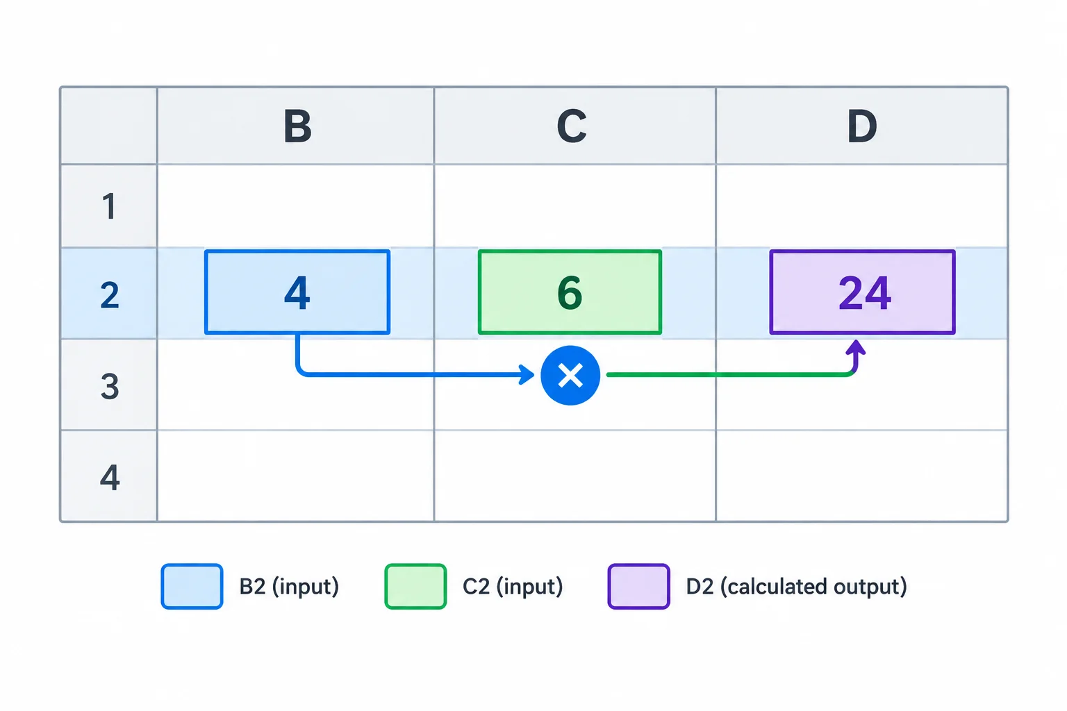
The formula in D2 uses two source cells and one arithmetic operation.
This is the formula stored in D2, not the value displayed after calculation.
=B2*C2A range names every cell from its first endpoint through its last endpoint. In D2:D5, the colon means “through,” so the range includes D2, D3, D4, and D5.
In English-language Google Sheets on the web, use =SUM(D2:D5) for total revenue in D6. It adds the numeric weekly revenue values in that one inclusive range. The same baseline formula also works in English-language Excel.
Keep syntax questions separate from calculation questions. In English-US conventions, decimal values use a decimal point. Function names and separators can vary by application language or locale, so check those settings if an otherwise sensible formula is rejected.
A colon defines a range. A comma or semicolon separates separate function arguments; it does not replace the colon in a range.
| Formula form | What it uses | Syntax check |
|---|---|---|
| =SUM(D2:D5) | One inclusive range | No argument separator is needed |
| =SUM(D2,D3) | Two individual cells | Comma in English-US |
| =SUM(D2;D3) | Two individual cells | Locale-dependent separator variant |
Match each formula part to its role in the Practice worksheet.
Tap an item and then its matching pair.
For English-language Google Sheets on the web using English-US conventions, complete the weekly revenue formula for D2 and the total-revenue formula for D6.
D2: B2C2
D6: =(D2D5)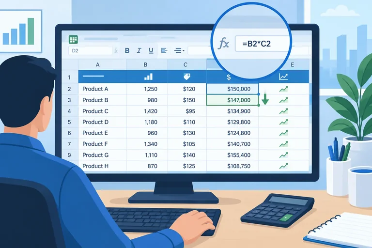
Step 4 of 8
Verify the first weekly revenue formula, then confirm that filling it down preserves the intended row-by-row logic.
In your own English-language Google Sheets spreadsheet on the web, open the Practice worksheet. Click D2, type the formula below, and press Enter.
Then compare the displayed result with your independent Week 1 check: 10 units at USD 5 each should produce USD 50.00. The formula is a suggestion to verify, not a result to trust automatically.
Enter this in cell D2.
=B2*C250
The unformatted numeric result is 50. If the cell is formatted as currency, it may display as USD 50.00.
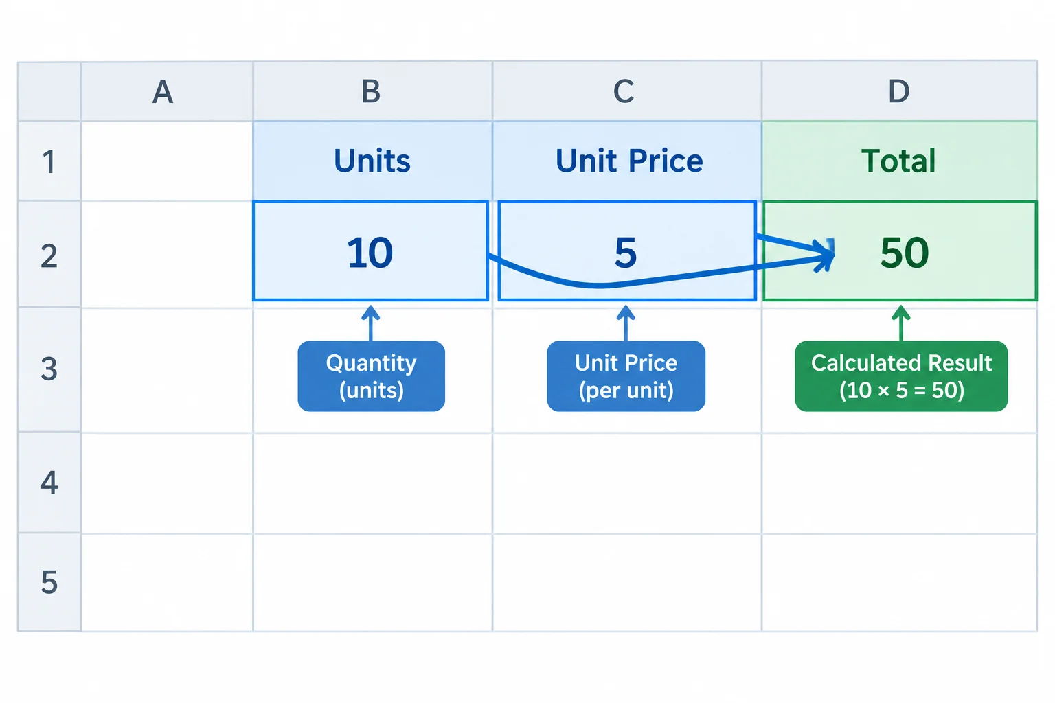
Check that D2 uses the Week 1 inputs, not just that it displays a plausible number.
A cell reference without dollar signs is a relative reference. When you fill a formula down one row, each reference shifts down one row too.
Select D2 and drag its fill handle down to D5. If needed, copy D2 and paste into D3:D5; the copied formulas should still shift relative references. Next, select D3 and inspect the formula bar or equivalent formula view—not only the number in the cell.
Week 2 has different inputs: 12 units and USD 5. Its result should be USD 60.00. This second-row check can reveal a formula that was correct in D2 but failed to shift after copying.
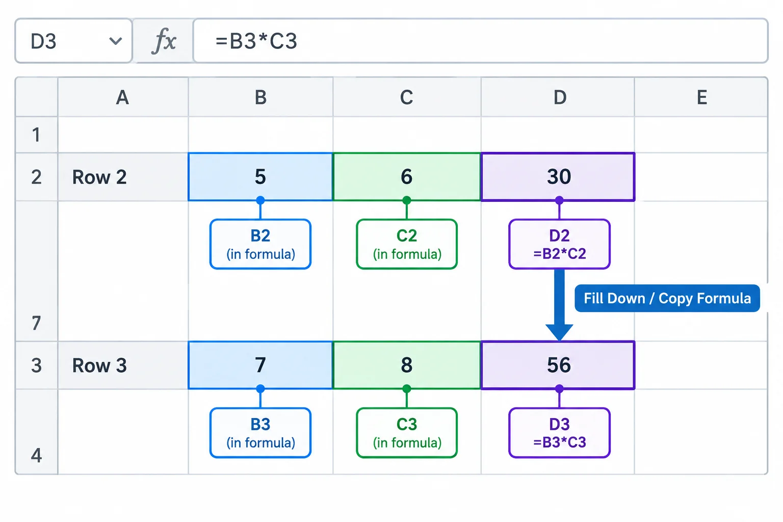
The formula text must change to the new row's inputs when it is filled down.
Tip
Displayed values alone are not enough. For example, a value can look reasonable by coincidence or because it still uses an earlier row. Inspect at least one copied cell in the formula bar and check both its references and its displayed result.
The formula in D2 was filled down exactly one row. Complete the formula that should appear in D3.
=*In your own Practice sheet, complete the fill-down check before responding. Record:
D2 and the displayed result you checked.D3 before filling down.D3, D4, or D5), its formula-bar text, and its displayed result.Write at least 120 characters (0/120).
Step 5 of 8
Validate spreadsheet totals by checking range coverage, selected columns, and an independent addition.
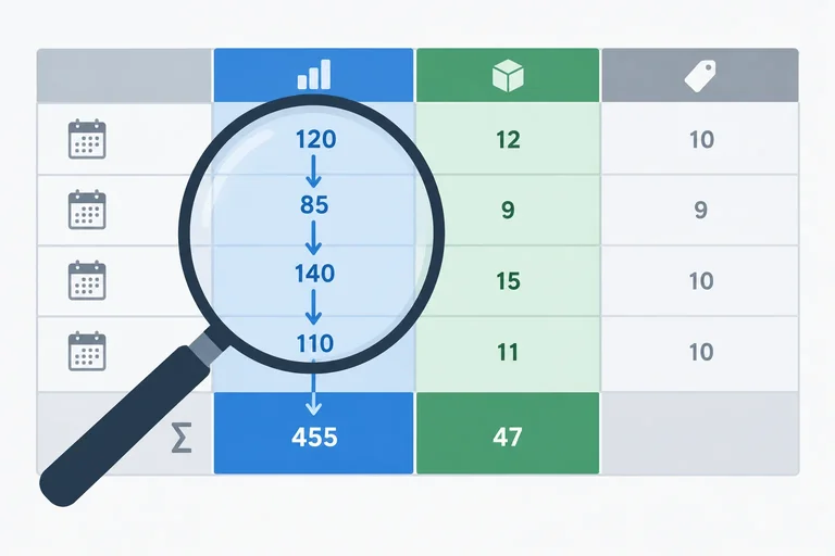
In Practice, rows 2–5 are the complete weekly records. Row 6 is the summary row: B6 totals units sold, while D6 totals revenue. C6 stays blank because unit price is an input, not a total for this task.
Treat a suggested total formula as a claim about two things: which column it uses and which first and last rows it includes. A displayed total alone cannot prove either one.
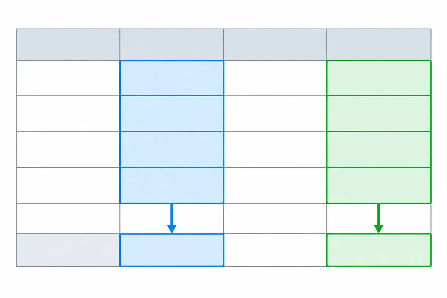
Check the selected column as well as both endpoints of a total range.
Use independent addition to check a spreadsheet total. The weekly revenue values are USD 50.00, USD 60.00, USD 80.00, and USD 100.00. A correct revenue total must agree with that addition, while the units total must be calculated from the separate units column.
The source cells and a manual check should point to the same result.
| Summary cell | Intended source cells | Independent check | Expected result |
|---|---|---|---|
| B6 | B2:B5 | 10 + 12 + 8 + 10 | 40 units |
| D6 | D2:D5 | 50 + 60 + 80 + 100 | USD 290.00 |
| C6 | None | Do not add prices | Blank |
Example
In English-language Google Sheets on the web, enter each formula separately in its named summary cell. The same formulas work in English-language Excel.
Enter the first formula in B6, then enter the second formula separately in D6.
Cell B6
=SUM(B2:B5)

Cell D6
=SUM(D2:D5)B6: 40 D6: 290
If D6 uses a currency display format, its numeric result may display as USD 290.00.
A total can be plausible but incomplete. In the separate Short range case, D6 contains =SUM(D2:D4). It adds USD 50.00 + USD 60.00 + USD 80.00, so it displays USD 190.00.
The formula is syntactically valid; its problem is coverage. Its ending reference stops before the Week 4 revenue row. Check the first endpoint, last endpoint, and column letter—not just whether the result looks believable.
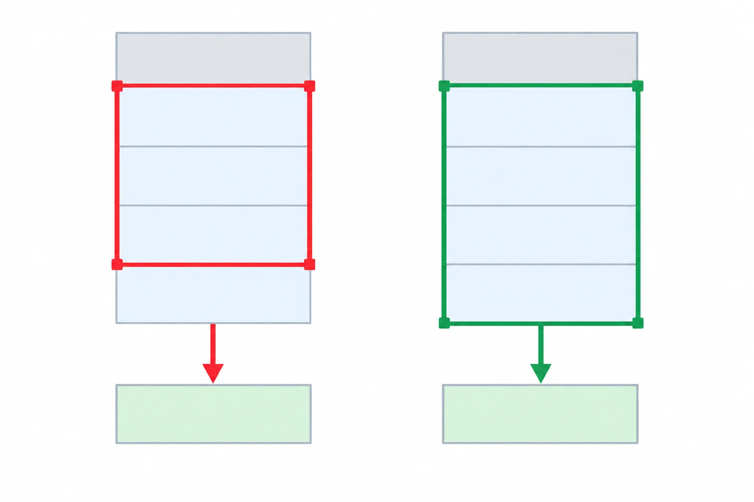
The faulty selection ends before the fourth weekly revenue cell; the correct selection includes every weekly row.
Tip
Keep diagnostic cases separate. The Short range case changes only the range in D6; the four weekly revenue values remain the baseline values. Restore the baseline before testing another kind of data problem.
Complete this diagnostic and repair check for the baseline Practice worksheet. Identify the omitted revenue cell, then complete the units and revenue ranges so each total covers all four weekly rows in the appropriate column.
Short range omitted:
B6: =SUM()
D6: =SUM()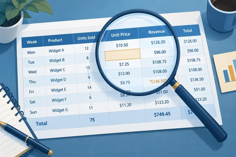
Step 6 of 8
Diagnose blank inputs and numeric-looking text entries without confusing them with an incorrect SUM range.
A surprising total is not always a range error. Start each diagnosis from the verified baseline in the Practice worksheet: D2:D5 contains revenue formulas and D6 totals that range.
Change only one thing at a time. After each check, restore the baseline before trying the next case. That makes the changed result traceable to one specific cause.
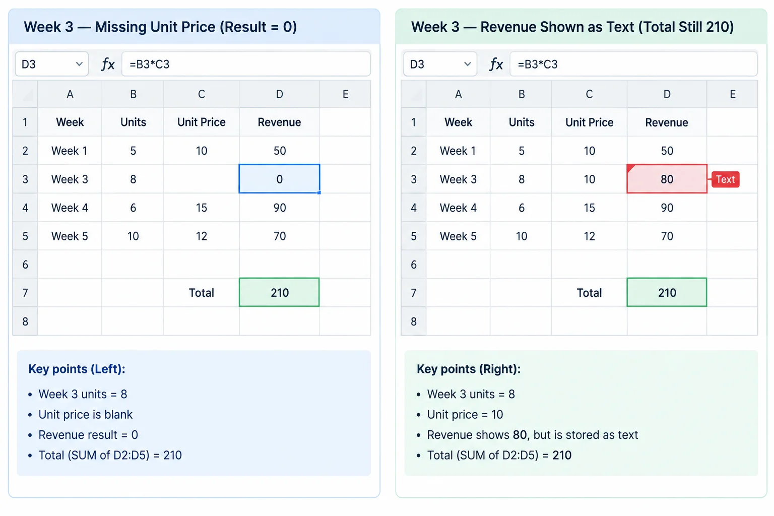
Both controlled cases can show USD 210.00, but the cells being excluded and the appropriate fixes differ.
Warning
Missing price is not evidence that the price was USD 0.00. In this case, clear C4 while keeping the formula in D4. The multiplication can display zero because a blank input participates in the calculation. Find the verified source price; do not invent a replacement.
Text revenue is different: restore the baseline, then replace the formula in D4 with the text entry '80. It may look like 80, but it is no longer a numeric formula result. SUM ignores text in referenced cells.
Check the cell itself, not just its appearance. In English-language Google Sheets on the web, select the suspicious cell and inspect the formula bar or cell contents. Also notice any application warning. A displayed value can hide a blank source input or a number stored as text.
For each controlled case below, restore the verified baseline before starting the next one. Keep D6 as =SUM(D2:D5) unless the case explicitly changes it.
Use these checks in your own Practice sheet. They separate an incomplete range from an input problem and from a displaced formula.
| Case | Single change | What to inspect | Appropriate next action |
|---|---|---|---|
| Short range | D6 uses `=SUM(D2:D4)` | Range endpoint and selected column | Restore the intended range through row 5 |
| Missing price | Leave `C4` blank | Contents of C4; formula remains in D4 | Seek the missing source price, then enter the verified value |
| Text revenue | Replace D4 with `'80` | Formula bar or cell contents; numeric status | Restore the formula in D4, then recalculate |
Match each controlled case to its cause and the appropriate correction.
Tap an item and then its matching pair.
In your own Practice worksheet, perform each controlled case separately and restore the baseline between them. Then write a compact check record:
Write at least 180 characters (0/180).

Step 7 of 8
Check an AI-generated trend explanation against comparable periods, consistent units, and the verified values in the Practice worksheet.
Before accepting a trend statement, compare like with like. In Practice, each row is one complete, consecutive seven-day period for the same product, so Week 1 through Week 4 can be compared as weekly periods.
Keep the measures separate:
Revenue rises in every consecutive weekly comparison. That observation does not by itself describe the pattern of units sold or explain why revenue changed.
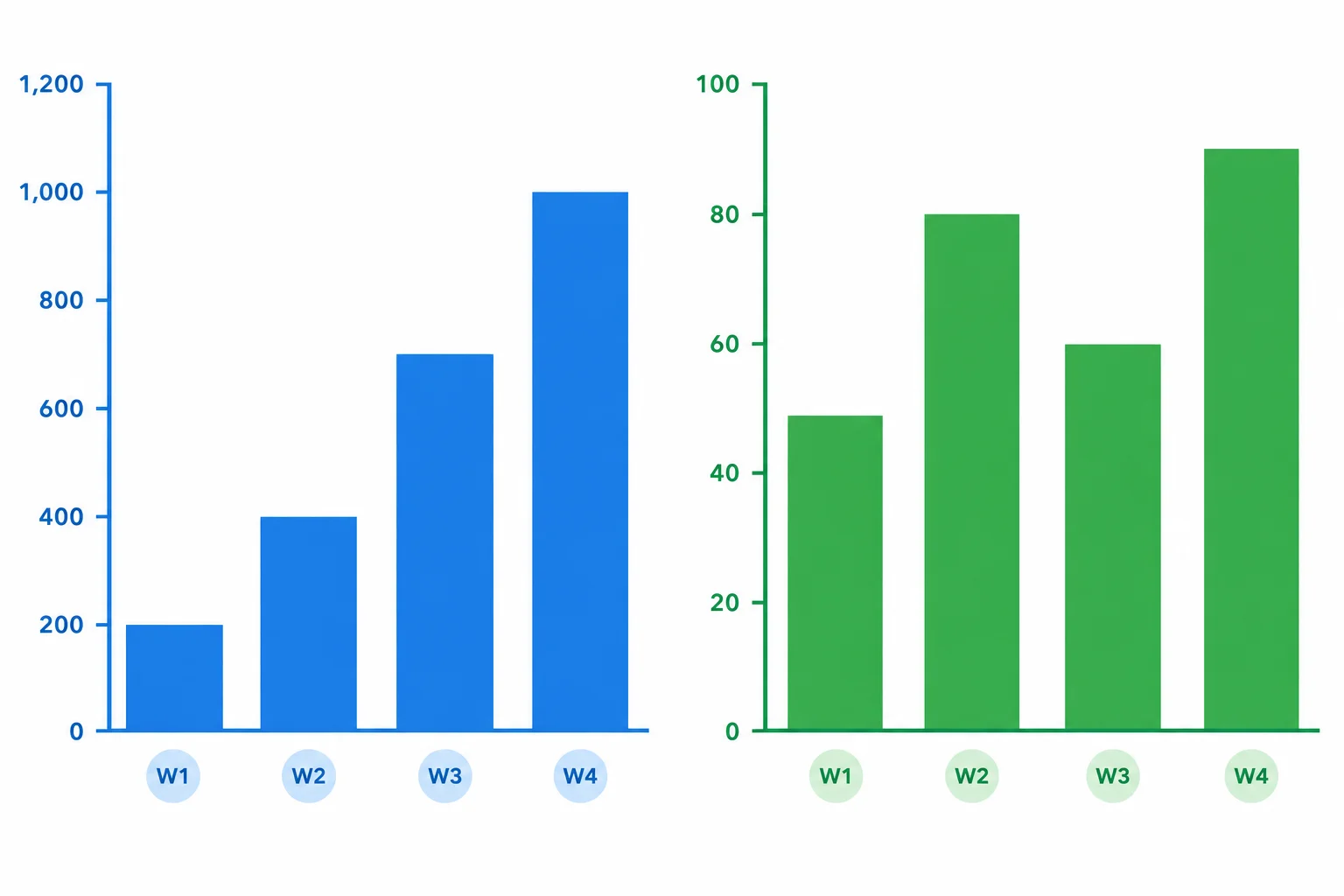
Use separate scales for revenue and units. Compare values within the same chart; do not infer that similarly shaped or sized bars across different measures mean the same thing.
A useful explanation says exactly what is being compared. A total answers a different question from a weekly value, even when both are revenue amounts.
Use the indicated cells as evidence before accepting a statement from an AI assistant.
| Type of statement | Evidence in Practice | Supported wording |
|---|---|---|
| Four-week revenue total | D6 = USD 290.00 | Revenue across all four weeks was USD 290.00. |
| First-to-last revenue | D2 and D5: USD 50.00, USD 100.00 | Week 4 revenue was USD 50.00 higher than Week 1. |
| Every weekly revenue change | D2:D5: 50, 60, 80, 100 | Revenue increased in each consecutive week. |
| Units pattern | B2:B5: 10, 12, 8, 10 | Units did not increase steadily. |
Example
AI draft: “Revenue rose every week, and units sold rose steadily. The change from USD 290.00 to USD 100.00 confirms the weekly trend.”
Checked version: Revenue did rise each week, from USD 50.00 to USD 60.00 to USD 80.00 to USD 100.00. Units did not rise steadily: they were 10, 12, 8, and 10. USD 290.00 is a four-week total, while USD 100.00 is one week, so they are not comparable as a single weekly change.
The table supports observations about values; it does not establish outside causes for the changes.
True or false: Because revenue increased in every week, units sold also increased in every week.
Review this AI draft about the baseline Practice table:
“Revenue improved because the four-week total changed from USD 290.00 to Week 4 revenue of USD 100.00. Units sold increased steadily along with revenue.”
Write a corrected explanation in 2–3 sentences. Include: (1) whether weekly revenue rose in every comparable period, with specific values; (2) the actual units pattern, with specific values; and (3) why the USD 290.00 and USD 100.00 comparison is invalid. State only what the table supports.
Write at least 120 characters (0/120).
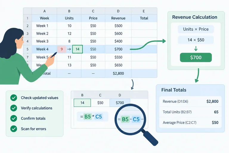
Step 8 of 8
Update a small spreadsheet table, verify formula suggestions against independent checks, and write an evidence-supported trend explanation.
Change only B5 in your local Practice worksheet from 10 to 14. Keep every other source value and every header unchanged.
Before asking an AI for anything, calculate the new checks independently. Week 4 revenue uses the updated units value and the existing Week 4 price. Then reconcile the two totals from all four weekly rows.
This order matters: an AI suggestion is only a candidate. It becomes a checked result after its references, coverage, and displayed values agree with your independent checks.
Use these values as independent checks after changing only B5. Monetary amounts are shown in USD for readability; numeric spreadsheet cells should remain numeric.
| Check | Cell | Expected value | Reason |
|---|---|---|---|
| Updated input | B5 | 14 | Week 4 units sold |
| Week 4 revenue | D5 | USD 140.00 | 14 × 10 |
| Total units | B6 | 44 | 10 + 12 + 8 + 14 |
| Total revenue | D6 | USD 330.00 | 50 + 60 + 80 + 140 |
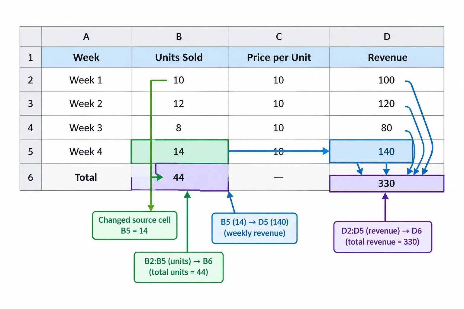
One source change should be traceable to its row calculation and both relevant totals.
Use a revised request that supplies enough context to test the response. For example:
“Using English-language Google Sheets on the web with an English-US formula locale, my worksheet is named Practice. Headers A1:D1 are Week, Units sold, Unit price (USD), and Revenue (USD). The values in A2:C5 are Week 1 | 10 | 5; Week 2 | 12 | 5; Week 3 | 8 | 10; Week 4 | 14 | 10. Give a formula for D2 that I can fill down through D5, a units-total formula for B6, and a revenue-total formula for D6. Use A1-style references. Explain the cells and operations used. I expect D5 to be 140, B6 to be 44, and D6 to be 330.”
The assistant cannot see or edit your sheet. Treat its answer as a suggestion to inspect in your own worksheet.
Candidate AI response to inspect
Enter in D2 and fill down through D5:
=B2*C2

Enter in B6:
=SUM(B2:B5)

Enter in D6:
=SUM(D2:D4)
Warning
The candidate also says: “Revenue rose every week because units sold increased every week. Total revenue is USD 330.00.”
Do not accept this statement because it sounds confident. Inspect the formula references and compare each trend claim with the updated weekly rows.
Summary
Repair the candidate’s total-revenue formula so its inclusive range covers every weekly revenue cell in D2:D5.
=SUM(D2:D)Create a concise completion record from your own updated Practice sheet. Include all four parts:
Practice worksheet, the changed B5 value, the formula destinations, and expected checks.D5, B6, and D6.Use values and cell references as evidence, not a general statement that the answer “looks right.”
Write at least 300 characters (0/300).
Congratulations! You completed: Requesting and Checking Spreadsheet Formulas
Thousands of online courses in video, ebooks and audiobooks.
To test your knowledge during online courses
Generated directly from your cell phone's photo gallery and sent to your email

Download our app via QR Code or the links below:.



Carry knowledge in your pocket.
Download the Cursa app.
There are hundreds of free courses available, with a free certificate of completion that is saved in your mobile image gallery.
Download the app to access the Course Completion Certificate for Free.


+ 10 million
students

Free and Valid
Certificate

60 thousand free
exercises

4.8/5 rating in
app stores

Free courses in
video and ebooks