
Exercises
Explore the numerical techniques physicists use when analytical solutions are unavailable. This quiz covers finite differences, numerical quadrature, Euler and Runge–Kutta methods, stability criteria, Monte Carlo error, boundary conditions, sparse matrices, FFTs, and symplectic integration. Questions combine conceptual understanding, formulas, convergence analysis, and visual interpretation of computational results.
Answer the questions below and check the explanation for each answer.
0/16 answered
Auto audio on: the next questions will be read aloud when you click Continue.
Very small steps reduce truncation error, but subtracting nearly equal floating-point values amplifies round-off error. An optimal step balances these two error sources.
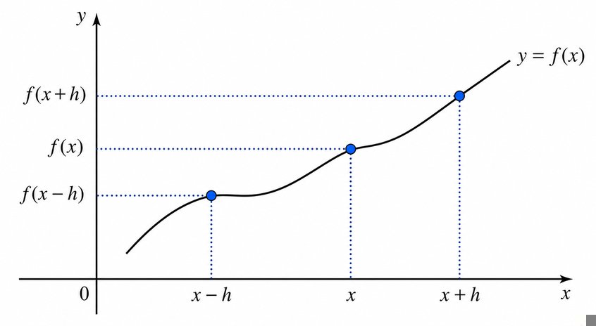
The centered first derivative uses samples equally spaced on both sides of x. Its truncation error is proportional to h².
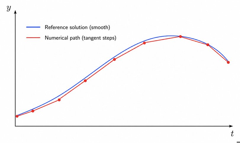
This is the explicit Euler method. It advances the solution using the derivative evaluated at the current point.
Euler's amplification factor is 1−hλ. Stability requires |1−hλ| < 1, which gives 0 < hλ < 2.
Classical RK4 calculates four slopes, commonly denoted k₁, k₂, k₃, and k₄, and combines them in a weighted average.
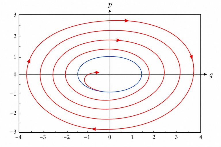
An ideal oscillator follows a closed phase-space orbit. An outward numerical spiral means the computed energy is increasing systematically even though the physical energy is constant.
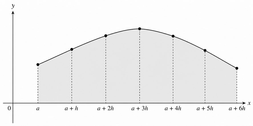
The trapezoidal rule gives half weight to the two endpoints and full weight to every interior sample.
Simpson's 1/3 rule has degree of precision three, so it exactly integrates constant, linear, quadratic, and cubic polynomials.
The standard error of an independent-sample mean decreases as 1/√N. Reducing the error by a factor of two therefore requires about four times as many samples.
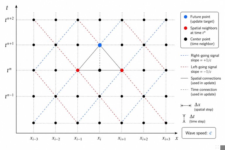
The Courant–Friedrichs–Lewy condition requires the numerical domain of dependence to include the physical one. For this scheme, the Courant number cΔt/Δx must not exceed one.
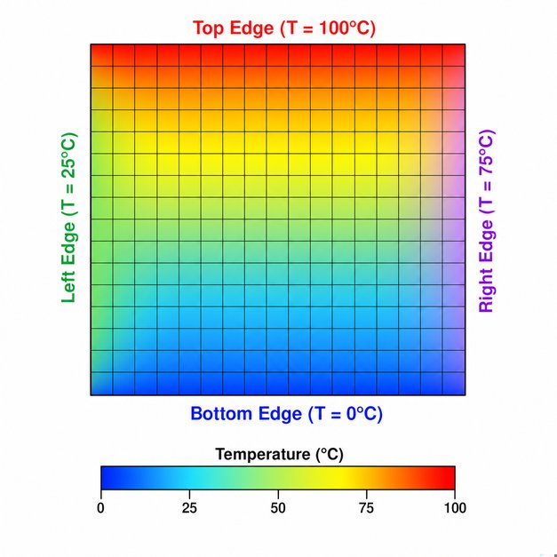
A Dirichlet condition specifies the value of the field itself at a boundary. A Neumann condition would instead specify its normal derivative or flux.
Local finite-difference stencils involve only neighboring grid values. Consequently, each matrix row has relatively few nonzero coefficients.
If E is proportional to h², replacing h with h/2 gives E/4. This scaling is commonly checked through grid-refinement studies.
Velocity Verlet first advances position with the current acceleration, evaluates the new acceleration, and then advances velocity using the average acceleration.
The FFT reorganizes the discrete Fourier transform to reduce its cost from direct O(N²) evaluation to approximately O(N log N).
Implicit schemes often have much larger stability regions. This permits time steps based on the desired accuracy rather than the fastest decaying timescale, although an algebraic solve is required.
Free CourseRelativity Course: Special and General Relativity, Tensors, Black Holes, Gravitational Waves and Cosmology
5

(3)

19h01m

39 exercises
Free CourseIntroduction to Thermodynamics
5
(1)
1h48m
9 exercises

Free CourseNuclear and Radiochemistry
5
(1)
31h56m
31 exercises
Free CoursePhysics for beginners
5
(1)
1h57m
2 exercises
Free CourseThermodynamics and Statistical Physics
5
(1)
14h53m
23 exercises
Free CourseAstrophysics and Cosmology Course
5
(1)
1h24m
5 exercises

Free CoursePhysics of Solar Energy Conversion
5
(4)
4h59m
16 exercises
Free CourseQuantum Physics
5
(1)
24m
4 exercises
Thousands of online courses in video, ebooks and audiobooks.
To test your knowledge during online courses
Generated directly from your cell phone's photo gallery and sent to your email

Download our app via QR Code or the links below:.



Carry knowledge in your pocket.
Download the Cursa app.
There are hundreds of free courses available, with a free certificate of completion that is saved in your mobile image gallery.
Download the app to access the Course Completion Certificate for Free.


+ 10 million
students

Free and Valid
Certificate

60 thousand free
exercises

4.8/5 rating in
app stores

Free courses in
video and ebooks