What a Forensic Timeline Is (and What It Is Not)
A forensic timeline is a structured view of events ordered by time, built from many independent data sources (file system timestamps, Windows event logs, application logs, cloud audit records, browser history, email headers, mobile artifacts, and more). The goal is to reconstruct “what happened, when, and in what order,” while also showing the confidence level and possible ambiguity of each timestamp.
A timeline is not a single authoritative truth. Different artifacts record time differently, with different precision, different time zones, and different opportunities for manipulation. A good timeline keeps the original timestamp values, records the assumed time zone, and documents any conversions or corrections applied so another examiner can reproduce your results.
Core Timeline Concepts: Event Time, Record Time, and Observation Time
Event Time vs. Record Time
Many artifacts store the time an event occurred (event time), but some store the time the event was written (record time) or last updated. For example, a security log entry might reflect when the system believes the event occurred, while a database entry might reflect when the application committed the transaction. When building a timeline, label which kind of time you are using and avoid mixing them without noting it.
Observation Time and Collection Time
Observation time is when you, the examiner, observed or collected the data (for example, when you exported a log or pulled a cloud audit report). This matters because some sources are mutable and can change between the incident and your collection. In your timeline notes, keep a small “collection metadata” record: when the artifact was collected, from where, by whom, and with what tool or method.
Precision and Granularity
Some timestamps are precise to milliseconds or microseconds, while others are only to the nearest second (or worse). When correlating events, do not assume two events with the same second-level timestamp happened simultaneously. Prefer ordering by higher-precision sources when available, and annotate the precision of each source.
- Listen to the audio with the screen off.
- Earn a certificate upon completion.
- Over 5000 courses for you to explore!

Download the app
Time Zones in Investigations: The Hidden Source of False Leads

Local Time, UTC, and “Display Time”
UTC is a time standard not affected by daylight saving time (DST). Many systems store timestamps in UTC and convert them for display based on the viewer’s time zone settings. Others store local time directly. A common mistake is to export logs in “local time” from one interface and compare them to UTC-based logs from another, creating apparent gaps or overlaps that are not real.
When you build a timeline, decide on a single “analysis time zone” for presentation (often UTC for cross-system cases) and convert everything to that zone while preserving the original values in separate fields.
Daylight Saving Time (DST) Pitfalls
DST can create duplicated or missing hours. For example, when clocks “fall back,” the hour from 01:00 to 02:00 occurs twice in local time. When clocks “spring forward,” an hour is skipped. If an incident occurs during a DST transition, local timestamps can appear out of order or ambiguous. In those cases, prefer UTC-based sources or sources that include an offset (for example, ISO 8601 timestamps like 2026-01-07T10:15:30-05:00).
Roaming Devices and Travel
Laptops and phones travel. A user may create artifacts in one time zone and later connect in another. Some systems update the time zone automatically; others do not. Your timeline should track time zone changes as events themselves when possible (for example, a configuration change, a mobile carrier update, or a system setting change). If you suspect travel, correlate with Wi-Fi networks, VPN endpoints, cellular tower regions, or cloud sign-in location metadata to validate the likely local time.
Where Time Comes From: System Clocks, NTP, and Domain Time
System Clock vs. Hardware Clock
Most computers have a hardware clock (RTC) and an operating system clock. The OS reads the hardware clock at boot and then maintains its own time. Misconfiguration can occur if the hardware clock is set to local time but the OS expects UTC (or vice versa). This can produce consistent offsets that affect file times and logs.
NTP and Time Synchronization
Network Time Protocol (NTP) is used to synchronize clocks. In enterprise environments, domain-joined Windows systems typically sync time with domain controllers, which in turn sync with a reliable upstream source. If time sync fails, systems can drift (time skew), causing log correlation errors. When investigating, you want to know: was the system synchronized, to what source, and how stable was the clock during the incident window?
Practical Checks for Time Sync Status
During live response (when permitted), you can query time configuration and status. On Windows, you can use built-in commands to capture time service details for later analysis.
REM Capture current time and time zone info (Windows) date /t time /t tzutil /g w32tm /query /status w32tm /query /configuration w32tm /query /peersSave outputs with the system name and collection time. These outputs help you estimate whether the machine was in sync and whether an offset is plausible.
Time Skew: Causes, Detection, and Controls
Common Causes of Time Skew
- Misconfigured time zone or DST settings.
- NTP disabled or blocked by firewall.
- Virtual machines paused/resumed or snapshotted, causing clock jumps.
- CMOS battery issues leading to drift or resets.
- Intentional tampering by an attacker or user to confuse logs.
- Dual-boot systems where one OS writes the hardware clock differently.
Detecting Skew by Cross-Referencing Independent Sources
Skew detection is about comparing timestamps that should align across independent systems. Examples include: a cloud sign-in event (server-side UTC) compared to a local interactive logon; an email sent time (server) compared to a file created time (local); or a VPN connection log compared to a local network connection event. If you see a consistent offset (for example, local events are always 7 minutes ahead), you may be dealing with clock drift rather than random discrepancies.
Be careful: not all differences are skew. Some are simply different time zones or different “event vs record” semantics. Your job is to determine whether the difference is systematic and explainable.
Time Skew Controls: How to Correct Without Destroying Meaning
“Time skew controls” are the methods you use to normalize timestamps for analysis while preserving the original evidence. The key principle is: never overwrite original timestamp values in your working dataset without keeping the raw value and the transformation you applied.
- Normalization: Convert all timestamps to a single analysis time zone (often UTC) and store the converted value in a separate field.
- Offset correction: If you can justify a consistent skew (for example, +420 seconds), apply an offset to create a “corrected time” field, but keep the uncorrected time too.
- Confidence scoring: Mark corrected times as “estimated” unless you have strong proof (like time service logs showing the exact offset).
- Windowed correlation: Instead of forcing exact matches, correlate events within a tolerance window (for example, ±2 minutes) when precision is low or skew is suspected.
Step-by-Step: Building a Multi-Source Timeline with Time Zone and Skew Handling
Step 1: Choose Your Timeline Standard Fields
Before importing data, define a consistent schema so you can merge sources cleanly. A practical minimum set of fields is:
- source (e.g., “Windows-SecurityLog”, “M365-Audit”, “Browser-History”)
- event_type (e.g., “logon”, “file_create”, “policy_change”)
- timestamp_raw (exact value as stored or exported)
- timestamp_raw_tz (what time zone/offset the raw value represents, if known)
- timestamp_utc (converted to UTC for sorting)
- timestamp_corrected_utc (optional: after skew correction)
- host/user (system and account context)
- details (short human-readable summary)
- confidence (high/medium/low, or numeric)
- notes (why you believe the time zone/skew assumption is valid)
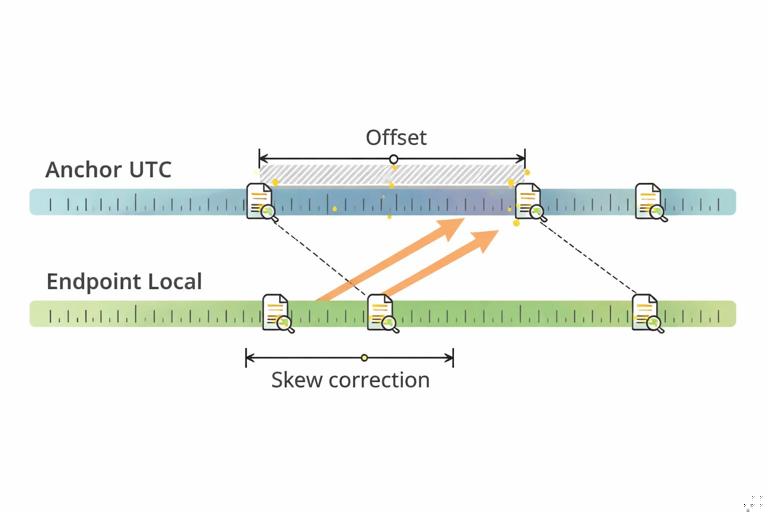
Step 2: Identify the “Anchor Sources”
Anchor sources are those most likely to have accurate time and clear time zone semantics. Common anchors include server-side cloud audit logs (usually UTC), email server logs, VPN concentrator logs, and domain controller logs. Pick at least one anchor for each environment involved (endpoint, identity provider, network, cloud).
Use anchors to establish a baseline: what time zone should your analysis use, and is there evidence the endpoint clock was drifting?
Step 3: Determine the Endpoint Time Zone at the Incident Time
Do not assume the current time zone equals the incident time zone. Look for evidence of time zone configuration and changes around the incident window. If you have multiple endpoints, do this per host. If you cannot prove it, record your assumption and treat conversions as provisional.
Practical approach: if local logs display local time without offset, but you also have at least one event that appears in both local and server logs (for example, a sign-in), you can infer the local offset by aligning the two.
Step 4: Convert Everything to UTC (Without Correcting Skew Yet)
First, do a pure time zone conversion. This step addresses “time zone mismatch,” not “clock drift.” Keep the raw timestamp untouched. If a source already provides UTC with an offset, store it as-is and compute UTC explicitly for sorting.
If you are using a spreadsheet or a scripting approach, ensure you are not accidentally applying your own workstation’s time zone during import. Many tools will interpret timestamps differently depending on locale settings.
Step 5: Test for Consistent Skew
Now compare endpoint-derived events to anchor events that should be near-simultaneous. Build a small table of pairings: event A (anchor) and event B (endpoint) that represent the same action. Compute the difference in seconds. If the differences cluster tightly (for example, always around +300 seconds), you likely have skew.
Example pairing ideas:
- Cloud sign-in success vs. local interactive logon or token acquisition event.
- VPN connection established vs. local network connection event.
- File upload recorded in cloud audit vs. local file access or archive creation time.
Step 6: Apply an Offset Correction Field (If Justified)
If you have strong evidence of a consistent skew, create a corrected timestamp field by applying the offset. Do not replace the UTC field; add a new one. Document the offset, the evidence used to derive it, and the time range for which it applies (skew can change over time).
# Example logic (pseudocode) corrected_utc = timestamp_utc - skew_seconds # if endpoint clock was fast by skew_secondsIf skew appears to change (for example, a sudden jump), treat it as multiple segments: “before adjustment” and “after adjustment.” This is common with virtual machines, manual clock changes, or NTP resynchronization events.
Step 7: Sort and Review with a Correlation Window
Even with corrections, do not overfit. Use a correlation window appropriate to your sources. For high-precision logs, you might use seconds. For low-precision artifacts, use minutes. When presenting the timeline, show the corrected time (if used) but keep the raw time visible for transparency.
Practical Example: Reconciling Endpoint Local Time with Cloud UTC

Scenario Setup
You have a cloud audit record showing a file was uploaded at 2026-01-07 14:10:00Z. On the endpoint, you find a local artifact indicating the archive was created at 09:12:30 (no offset shown). The user is believed to be in Eastern Time (UTC-5) in January (no DST). If the endpoint clock is correct, 09:12:30 local corresponds to 14:12:30Z, which is 150 seconds after the upload time—possible if the archive creation time reflects last write completion and the upload log reflects start time, or if one is record time.
But you also find a second pairing: cloud sign-in at 13:00:00Z and local logon at 08:03:00 local, which converts to 13:03:00Z. Now you have a consistent +180 seconds difference. That suggests the endpoint clock is slow by about 3 minutes (or the local artifact times are recorded late). With multiple pairings showing the same offset, you can justify adding a corrected time field for endpoint events: timestamp_corrected_utc = timestamp_utc - 180 seconds.
How to Document This in the Timeline
In the timeline row notes, record: “Local timestamps appear ~+180s relative to cloud anchor events; corrected_utc computed by subtracting 180s; evidence: sign-in pairing A/B, upload pairing C/D.” Mark confidence as medium unless you have direct time service evidence showing the offset.
Handling Ambiguous or Missing Time Zone Information
When a Log Export Loses Offset Information
Some exports produce timestamps like “01/07/2026 09:12:30” without specifying time zone. In that case, treat the time zone as unknown until you can infer it. Store timestamp_raw exactly as given and set timestamp_raw_tz to “unknown.” Only populate timestamp_utc once you have a defensible assumption.
When Different Tools Render the Same Data Differently
It is common for one tool to display a timestamp in local time and another to display the same underlying value in UTC. To prevent confusion, record the tool name and its display settings when you export. If possible, export in a standardized format that includes offset (ISO 8601) or explicitly choose UTC in the export options.
Quality Controls for Timeline Reliability
Keep a “Time Assumptions” Ledger
Create a small section in your case notes (or a separate worksheet) listing each host and source with: assumed time zone, evidence supporting it, whether DST applies, and whether skew correction was applied. This prevents silent assumptions from creeping into your analysis.
Spot Checks and Sanity Tests
Perform quick sanity tests: do daily patterns make sense (work hours vs. midnight activity)? Do sequences align with known external events (ticket submissions, emails, meeting times)? If a timeline suggests impossible ordering (a response before a request), re-check time zones, DST, and record-vs-event semantics before assuming tampering.
Present Both Raw and Normalized Time in Reports
When you later present findings, show normalized UTC for readability and cross-system correlation, but include raw time and the original source context. This reduces disputes and makes your work reproducible if another examiner needs to validate the timeline.