What a “Simple Time-Series Forecast” Means in Operations
In operations, a time-series forecast is a prediction of future demand or workload based on past values observed over time (daily orders, weekly tickets, hourly call volume, monthly shipments, etc.). “Simple” does not mean careless; it means using methods that are easy to explain, quick to maintain, and robust enough for day-to-day planning. The goal is usually not perfect accuracy—it is to produce a usable baseline that helps you staff shifts, plan inventory, schedule production, or anticipate backlog risk.
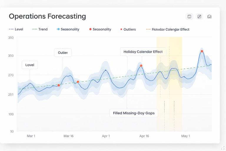
Time-series forecasting is different from “driver-based” forecasting (where you model demand from inputs like marketing spend or price). In a time-series approach, the main signal is the historical pattern itself: level (typical value), trend (up/down movement), and seasonality (repeating cycles like day-of-week or month-of-year). In operations, you often also deal with calendar effects (holidays, end-of-month spikes), missing days, and outliers (system outage, one-time bulk order). Simple methods handle these realities by focusing on stable patterns and by using guardrails to avoid overreacting to noise.
Common operational use cases
Workforce planning: forecast daily tickets to set staffing targets and on-call coverage.
Warehouse workload: forecast inbound pallets or outbound lines to plan labor and dock appointments.
Maintenance demand: forecast weekly work orders to balance preventive vs corrective capacity.
Continue in our app.- Listen to the audio with the screen off.
- Earn a certificate upon completion.
- Over 5000 courses for you to explore!

Download the app
Procurement and replenishment: forecast weekly consumption to set reorder points and safety stock reviews.
Data Requirements and Preparation (Forecast-Ready Time Series)
Before choosing a method, make sure your time series is forecast-ready. You do not need a complex model, but you do need consistent time indexing.
1) Choose the time grain that matches decisions
Pick the smallest time unit that your operational decision uses. If you staff by day, forecast by day. If you plan production weekly, forecast weekly. Avoid forecasting at a finer grain than you can act on, because noise increases and accuracy typically drops.
2) Ensure a complete calendar (no missing periods)
A common operational pitfall is missing dates: days with zero demand are absent rather than recorded as 0. Forecast methods interpret missing periods as “unknown,” which can distort averages and seasonality. Build a complete calendar and left-join your actuals onto it so every date exists, with blanks converted to 0 (or to an imputed value if 0 is not valid for your metric).
3) Decide how to treat outliers
Simple forecasts are sensitive to extreme spikes. In operations, spikes may be real (promotion) or non-repeatable (one-time bulk order). Decide a rule: cap at a percentile, replace with a rolling median, or flag and exclude from the baseline. The key is consistency and auditability: you should be able to explain why a point was adjusted.
4) Separate “actuals” from “forecast” and “plan”
Keep actuals as the source signal. Forecasts are derived outputs. If you overwrite actuals with forecasts, you lose the ability to evaluate accuracy and improve. In the worksheet, keep a clean series of actuals and then add forecast columns alongside.
Method 1: Naive and Seasonal Naive (Fast Baselines)
The simplest forecast is “tomorrow equals today.” This is surprisingly effective for stable processes with low trend and low seasonality. A better operational baseline is often seasonal naive: “next Monday equals last Monday,” “next week equals the same week last year,” etc.
When to use
Demand is stable with repeating cycles (day-of-week patterns, weekly cycles).
You need a quick baseline for staffing or capacity checks.
You want a benchmark to compare more advanced methods against.
Step-by-step in Excel (daily data with weekly seasonality)
Assume you have a table with columns: Date and Actual, one row per day. You want a forecast for the next 14 days.
Naive: Forecast for day t+1 equals Actual at day t.
Seasonal naive (weekly): Forecast for day t equals Actual from 7 days earlier.
In a forecast column (for dates beyond the last actual), you can reference the value 7 rows above if your table is strictly daily with no gaps. If gaps exist, use a lookup by date (date minus 7 days) rather than row offset.
SeasonalNaiveForecast = value on (Date - 7)Operational tip: seasonal naive is often a strong baseline for call centers, ticket queues, and warehouse shipping where day-of-week effects dominate.

Method 2: Moving Average (Smoothing Noise)
A moving average forecast uses the average of the last N periods as the next period’s forecast. It smooths random variation and is easy to explain: “We forecast next week based on the average of the last 4 weeks.”
Choosing the window (N)
Short window (e.g., 7 days): more responsive, less smooth.
Long window (e.g., 28 days): smoother, slower to react to real changes.
Match N to the operational rhythm. For daily demand with weekly seasonality, a 28-day moving average often balances stability and responsiveness.
Step-by-step in Excel (rolling average baseline)
For each date, compute the average of the previous N actuals. Use that as the forecast for the next period. If you are forecasting multiple future periods, you can either keep using the last N actuals (static baseline) or roll forward using forecasts once actuals end (recursive). For operational dashboards, a static baseline is often preferred because it is easier to audit and does not compound error as quickly.
MovingAverageForecast(t+1) = AVERAGE(Actual(t-N+1) ... Actual(t))If you need a weekly forecast from daily data, consider aggregating to weekly totals first, then applying a moving average on weekly totals. This reduces noise and aligns with weekly staffing and capacity decisions.
Method 3: Weighted Moving Average (More Weight on Recent Periods)
A weighted moving average assigns higher weights to recent periods. This is useful when the process is changing (new product adoption, policy change, gradual volume growth) but you still want a simple method.
Example weighting scheme
Suppose you forecast next week’s tickets using the last 4 weeks with weights 0.4, 0.3, 0.2, 0.1 (most recent gets 40%).
Forecast = 0.4*Week(-1) + 0.3*Week(-2) + 0.2*Week(-3) + 0.1*Week(-4)Operational tip: keep weights simple and documented. Avoid “mystery weights” that no one can defend during planning meetings.
Method 4: Exponential Smoothing (Simple, Strong, and Maintainable)
Exponential smoothing is a widely used simple forecasting method. It produces a smoothed level where recent observations matter more than older ones, controlled by a parameter alpha (α) between 0 and 1.
Single exponential smoothing (SES)
SES is best for series with no strong trend or seasonality. It updates a smoothed value each period:
Level_t = α*Actual_t + (1-α)*Level_(t-1)The forecast for the next period is the latest level:
Forecast_(t+1) = Level_tHow to pick α in operations
Higher α (0.4–0.7): reacts quickly to changes; more volatile.
Lower α (0.1–0.3): stable; slower to react.
A practical approach is to test a small set of α values (for example 0.2, 0.3, 0.5) and select the one with the lowest error on recent history (see the accuracy section below). Keep the chosen α fixed for a period (e.g., a quarter) to avoid constant tuning.
Step-by-step in Excel (SES column setup)
Step 1: Create a column Level.
Step 2: Initialize the first level. Common choices: first actual value, or average of the first 7/14 days.
Step 3: For each subsequent row, compute Level using the formula above.
Step 4: Forecast for the next day equals the latest Level.
This method is easy to audit because each row depends only on the previous level and the current actual.
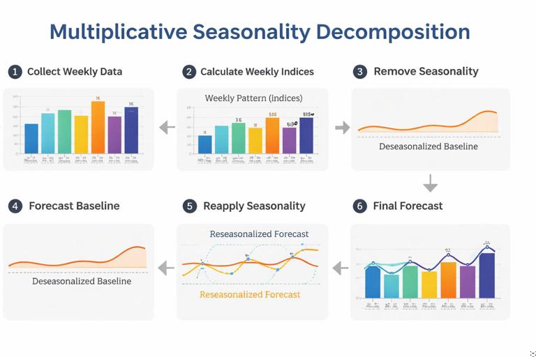
Handling Seasonality Without Complex Models
Many operational series have seasonality: day-of-week patterns, month-end spikes, or quarterly cycles. If you want to stay “simple,” you can handle seasonality with straightforward decomposition ideas: estimate seasonal factors, de-seasonalize, forecast the underlying level, then re-apply seasonality.
Seasonal indices (multiplicative approach)
Multiplicative seasonality assumes the seasonal effect scales with the level (e.g., Mondays are 20% higher than average). This is common in demand and workload.
Step-by-step outline (day-of-week indices):
Step 1: Compute the overall average of Actual over a stable historical window (e.g., last 8–12 weeks).
Step 2: Compute average Actual for each day of week (Mon, Tue, …) over the same window.
Step 3: Seasonal index for each day = (day-of-week average) / (overall average).
Step 4: De-seasonalize each day: Deseasonalized = Actual / SeasonalIndex(day).
Step 5: Forecast the deseasonalized series using a simple method (moving average or SES).
Step 6: Re-seasonalize the forecast: Forecast = BaseForecast * SeasonalIndex(future day).
This approach is explainable in operational reviews: “We forecast the underlying baseline volume, then apply the typical day-of-week pattern.”
Additive seasonality (when differences are constant)
If Mondays are consistently +30 tickets rather than +20%, additive indices may fit better. The process is similar, but you use differences instead of ratios:
AdditiveIndex(day) = DayAvg - OverallAvgDeseasonalized = Actual - AdditiveIndex(day)Forecast = BaseForecast + AdditiveIndex(future day)Choose multiplicative vs additive by inspecting whether peaks grow as the overall level grows (multiplicative) or stay roughly the same size (additive).
Forecast Accuracy for Operations: Simple Metrics You Can Trust
Forecasts should be evaluated with metrics that match operational decisions. A method that looks good on average may still fail on peak days, which are often the days that cause SLA breaches.
Key accuracy metrics
MAE (Mean Absolute Error): average of |Actual − Forecast|. Easy to interpret in units (tickets, orders).
RMSE (Root Mean Squared Error): penalizes large misses more heavily; useful when spikes are costly.
MAPE (Mean Absolute Percentage Error): average of |error|/Actual. Be careful when Actual can be near zero.
Bias (Mean Error): average of (Actual − Forecast). Shows systematic under-forecasting or over-forecasting.
Step-by-step: set up a backtest window
To compare methods fairly, simulate how the forecast would have performed historically.
Step 1: Choose a backtest period (e.g., last 8 weeks).
Step 2: For each day in the backtest, generate a forecast using only data available before that day (no peeking).
Step 3: Compute errors and aggregate metrics.
Step 4: Compare methods: seasonal naive vs moving average vs SES vs deseasonalized+SES.
Operational tip: track accuracy separately for weekdays vs weekends, or for peak seasons vs normal weeks. A single metric can hide important failure modes.
Forecast Horizons: Next Day vs Next Week vs Next Month
Simple methods behave differently depending on horizon.
Short horizon (1–7 days)
Seasonal naive often performs very well if day-of-week patterns are stable.
SES with a moderate α can adapt to small shifts.
Medium horizon (2–8 weeks)
Moving averages and weighted moving averages provide stable baselines.
Deseasonalize + SES can help if seasonality is strong.
Longer horizon (monthly/quarterly)
Simple time-series methods can still provide a baseline, but uncertainty increases. For operational planning, it is often better to present a baseline plus a range (see prediction intervals below) and to refresh frequently as new actuals arrive.
Prediction Intervals (Operational Ranges, Not Just Point Forecasts)
Operations rarely need a single number; they need a range to plan capacity buffers. A simple way to create a range is to use recent forecast errors to estimate variability.
Step-by-step: build a basic interval from recent MAE
Step 1: Compute absolute errors over a recent window (e.g., last 28 days) for your chosen method.
Step 2: Compute MAE over that window.
Step 3: Create an interval: Lower = Forecast − k*MAE, Upper = Forecast + k*MAE.
Choose k based on how conservative you want to be (k=1 is a moderate buffer; k=2 is more conservative). This is not a statistically perfect confidence interval, but it is practical and easy to explain: “Our typical miss is about X; we plan within ±2X.”
Calendar Effects: Holidays, Closures, and Month-End Spikes
Simple models struggle with calendar effects unless you explicitly handle them. In operations, these effects are often known in advance, so you can incorporate them as adjustments.
Holiday handling patterns
Option A: Exclude holidays from baseline calculations: remove those dates when computing averages and seasonal indices, then forecast normally and apply a manual adjustment for the holiday.
Option B: Use “like-for-like” mapping: forecast a holiday based on the same holiday last year (or the nearest comparable day).
Option C: Treat closures as zeros but flag them: if the operation is closed, demand may be zero but workload may shift to adjacent days; consider redistributing volume if that is typical.
Month-end and quarter-end effects
If you see consistent spikes at month-end, day-of-week indices alone will not capture them. A simple approach is to add a second set of indices for “day-of-month bucket” (e.g., days 1–25 normal, days 26–end elevated) or to flag the last 3 business days as a special category and compute an uplift factor from history.
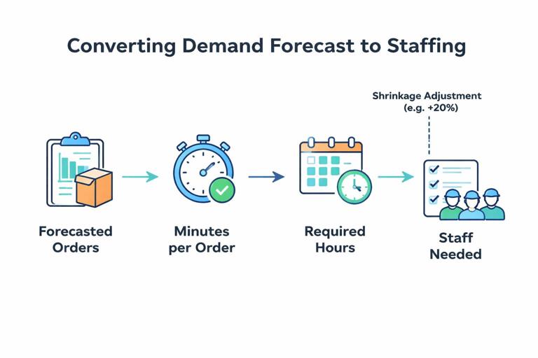
From Demand Forecast to Workload Forecast (Units, Time, and Capacity)
Operational workload is often not the same as demand. A forecast of orders becomes a forecast of labor hours after you apply productivity assumptions (minutes per order, pick lines per hour, tickets per agent hour). Keep the transformation explicit so planners can see what drives staffing.
Step-by-step: convert forecasted volume into required hours
Step 1: Forecast volume (e.g., orders/day).
Step 2: Apply average handling time or standard minutes (e.g., 6 minutes/order).
Step 3: Compute required minutes = ForecastVolume * MinutesPerUnit.
Step 4: Convert to hours and apply shrinkage/availability (breaks, meetings, absenteeism) if relevant.
RequiredHours = ForecastUnits * MinutesPerUnit / 60 / (1 - ShrinkageRate)Operational tip: if handling time changes with volume (congestion, batching), keep separate productivity assumptions for low/normal/peak days, or use a simple piecewise rule.
Practical Build: A Simple Forecast Block You Can Reuse
The following structure works well for many operational dashboards and trackers because it keeps the logic modular and testable.
1) Inputs (parameters)
Forecast horizon (e.g., 14 days)
Method selector (Seasonal Naive / Moving Avg / Weighted MA / SES / Deseasonalized+SES)
Window length (N) for averages
Alpha (α) for SES
Seasonality type (None / Day-of-week multiplicative / additive)
Outlier handling rule (None / cap / exclude flagged)
2) Helper calculations
Calendar completeness check (identify missing dates)
Day-of-week label for each date
Seasonal indices table (if used)
Deseasonalized actuals (if used)
3) Forecast engine
Implement each method in its own column so you can compare them side-by-side. Then use the method selector to pick which forecast feeds the dashboard. This avoids rewriting formulas and makes it easy to backtest.
4) Accuracy block
Compute MAE, RMSE, and bias over a rolling backtest window. Display them near the method selector so the user sees the trade-off between responsiveness and stability.
5) Output block
Point forecast for each future date
Upper/lower range based on recent error
Converted workload (hours) using productivity assumptions
Common Failure Modes and How to Keep Forecasts Operationally Useful
Failure mode: mixing partial days with full days
If today is incomplete (midday), including it as an “actual” will pull forecasts down. Use a rule: only include completed periods in the model. For intraday operations, forecast at the intraday grain (hourly) or exclude the current partial period.
Failure mode: structural change (new system, new policy)
When a process changes, older data may no longer represent the current reality. Simple fixes include shortening the training window (use last 4–8 weeks instead of last year) or resetting the SES level after the change date.
Failure mode: seasonality drift
Day-of-week patterns can change (e.g., more weekend orders after a service change). Recompute seasonal indices on a rolling basis (like last 8–12 weeks) rather than using a fixed index from long ago.
Failure mode: “forecasting the backlog” instead of arrivals
For ticket queues, you may have two series: arrivals (new tickets) and completions (resolved tickets). Forecast arrivals to plan staffing; forecast backlog separately using a simple flow balance: Backlog(t+1) = Backlog(t) + Arrivals(t+1) − Capacity(t+1). Mixing these concepts leads to confusing plans.