Forecasting and Capacity Planning with Scenarios and What-If Analysis

Why scenarios and what-if analysis matter in operations forecasting

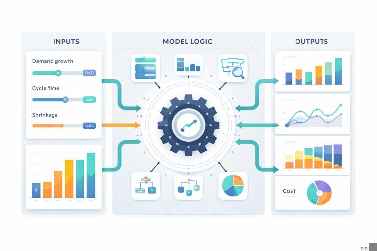
Operations forecasting is rarely about finding a single “correct” number. It is about understanding how demand, productivity, lead times, and constraints interact, then preparing plans that remain workable when reality deviates from assumptions. Scenarios and what-if analysis let you model uncertainty explicitly: you define a set of controllable assumptions (inputs), connect them to a forecast and capacity model (logic), and compare outcomes (outputs) such as required headcount, overtime hours, backlog, service level, or cost.

In Excel, scenario-based planning becomes powerful when you treat the model like a simulator: change a few drivers and immediately see the impact on capacity and performance. This chapter focuses on building a forecasting and capacity planning model that supports multiple scenarios, sensitivity checks, and goal-seeking decisions without rewriting formulas each time.

Core concepts: drivers, constraints, and planning horizons

1) Demand drivers vs. capacity drivers

Separate what creates work from what processes work.

• Demand drivers: forecasted order volume, tickets, shipments, production units, call arrivals, etc. Often expressed by time period (day/week/month) and by segment (product family, channel, region).

• Capacity drivers: available labor hours, machine hours, throughput rate, yield, uptime, staffing, shift patterns, learning curves, and planned downtime.

  Continue in our app.

  You can listen to the audiobook with the screen off, receive a free certificate for this course, and also have access to 5,000 other free online courses.

  Or continue reading below...

  

  Download the app

Good what-if analysis changes drivers, not hard-coded results. For example, you change “volume growth” or “cycle time” and the model recalculates “required FTE” and “expected backlog.”

2) Constraints and bottlenecks

Capacity planning is constrained by the tightest resource. If you have multiple steps (pick, pack, ship), the bottleneck step determines throughput. Your model should calculate capacity per step and highlight which step is limiting under each scenario.

3) Time buckets and the planning horizon

Choose time buckets that match operational decisions:

• Weekly for staffing and scheduling decisions.

• Monthly for budget and hiring plans.

• Daily for short-term dispatching and backlog burn-down.

For scenario planning, weekly is often a practical balance: enough detail to see peaks, not so granular that the model becomes fragile.

Model structure for scenario-based forecasting

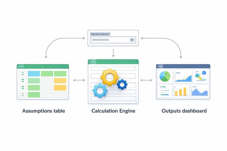
This chapter assumes you already have clean, structured data and reliable calculation patterns. Here, focus on organizing the planning model into three zones:

• Assumptions: scenario inputs (growth rates, productivity, shrinkage, overtime limits, lead times).

• Engine: forecast and capacity calculations by period and by resource/step.

• Outputs: KPIs, charts, and scenario comparisons (required capacity, gap, cost, service level).

The key is that the Engine references Assumptions through a scenario selector, so switching scenarios updates everything.

Step-by-step: build a scenario table and selector

Step 1: Create a scenario assumptions table

Create a table named tblScenarios with one row per scenario and one column per assumption. Example columns:

• Scenario (Base, High Demand, Low Demand, Labor Shortage, Productivity Gain)

• Demand_Growth (e.g., 0.03 monthly)

• Seasonality_Multiplier (e.g., 1.00 base, 1.15 peak)

• CycleTime_Minutes (e.g., 6.5 minutes per unit)

• HoursPerFTE_PerWeek (e.g., 37.5)

• Shrinkage (e.g., 0.12 for breaks, meetings, absence)

• Overtime_MaxPct (e.g., 0.10)

• Target_ServiceLevel (e.g., 0.95)

• Hiring_Lag_Weeks (e.g., 6)

Keep assumptions measurable and directly tied to operations. Avoid mixing “results” (like required FTE) into this table.

Step 2: Add a scenario selector cell

Create a single input cell (for example, named range selScenario) where the user chooses a scenario name. This cell will drive all assumption lookups.

Step 3: Pull scenario values into named assumption cells

Create a small assumptions panel with labels and formulas that retrieve the selected scenario’s values. Use a lookup keyed on Scenario. Example pattern (conceptually): “get the value from tblScenarios where Scenario = selScenario and return the column.”

For example, for Demand_Growth you retrieve the selected row’s Demand_Growth. Repeat for each assumption. This makes the Engine formulas simpler: they reference a single “current” assumption value rather than repeating lookups everywhere.

Step-by-step: build a demand forecast with scenario drivers

Step 1: Set up a time series table

Create a table named tblPlan with one row per week (or month). Suggested columns:

• PeriodStart

• Base_Demand (starting forecast before scenario adjustments)

• Seasonality_Index (1.00 normal, >1 peak, <1 trough)

• Scenario_Demand

Base_Demand can come from your existing forecast method (for example, a baseline from historical averages or a separate forecasting sheet). The scenario layer should adjust it, not replace it.

Step 2: Apply growth and seasonality

Scenario_Demand should incorporate scenario growth and seasonality. A common approach:

• Apply a growth factor over time (compounded by period).

• Multiply by a seasonality index (either from a table or a simple pattern).

Example logic in words: Scenario_Demand = Base_Demand × (1 + Demand_Growth)^(period_number) × Seasonality_Index × Seasonality_Multiplier.

This lets you create scenarios like “same baseline but 8% higher demand during peak weeks” without changing the baseline forecast.

Step-by-step: convert demand into workload hours

Step 1: Define workload per unit

Workload is demand translated into required effort. For a single-step process, a simple conversion is:

• Workload_Hours = Scenario_Demand × CycleTime_Minutes ÷ 60

If you have multiple steps (e.g., Receive, Pick, Pack), create a small table of step times and calculate workload per step. This is where bottlenecks become visible: each step has its own workload and capacity.

Step 2: Include rework, yield, or complexity mix

Many operations have non-linear workload drivers. Add columns for:

• Rework rate: extra work as a percentage of volume.

• Complexity mix: weighted average cycle time based on product mix.

• Yield: if only a portion of work completes successfully, effective workload increases.

Example in words: Effective_CycleTime = Base_CycleTime × (1 + ReworkRate) × MixFactor.

Step-by-step: calculate available capacity and required FTE

Step 1: Compute net available hours per FTE

Gross hours per FTE per week are reduced by shrinkage (breaks, meetings, training, absence). Net hours:

• NetHoursPerFTE = HoursPerFTE_PerWeek × (1 − Shrinkage)

This is a critical assumption: small changes in shrinkage can materially change required staffing.

Step 2: Convert workload hours into required FTE

For each period:

• Required_FTE = Workload_Hours ÷ NetHoursPerFTE

If you allow overtime, treat it as additional capacity, but cap it:

• MaxOvertimeHours = CurrentFTE × HoursPerFTE_PerWeek × Overtime_MaxPct

• EffectiveCapacityHours = (CurrentFTE × NetHoursPerFTE) + MaxOvertimeHours

Then compare EffectiveCapacityHours to Workload_Hours to calculate a capacity gap.

Step 3: Model hiring lag and ramp

Capacity planning is not only “how many FTE do we need,” but “when do we need them.” Add a hiring plan table with planned hires by week and apply a lag:

• Hires in week t become available in week t + Hiring_Lag_Weeks.

You can also model ramp-up (new hires at 50% productivity for first 2 weeks). Add a ramp factor by tenure and apply it to the effective FTE contribution.

Backlog and service level: turning capacity gaps into operational outcomes

Forecasting and capacity planning become more actionable when you translate capacity gaps into backlog and service impact.

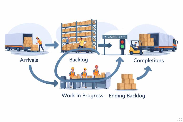
Backlog flow model

Create columns in tblPlan:

• Starting_Backlog

• Arrivals (Scenario_Demand)

• Completions (limited by capacity)

• Ending_Backlog

Completions can be modeled as the minimum of Arrivals + Starting_Backlog and Capacity_Units (capacity expressed in units). Convert capacity hours to units using cycle time.

Ending_Backlog = Starting_Backlog + Arrivals − Completions. Starting_Backlog for each period equals the prior period’s Ending_Backlog.

Service level approximation

If you have a service target like “95% completed within the week,” you can approximate service level using backlog ratio:

• If Ending_Backlog grows, service level deteriorates.

A simple operational KPI is Backlog Weeks = Ending_Backlog ÷ AverageWeeklyDemand. This expresses how many weeks of work are waiting, which is intuitive for planning discussions.

What-if analysis tools: Data Tables, Goal Seek, and Solver

One-variable and two-variable Data Tables for sensitivity

Data Tables are ideal when you want to see how outputs change across a range of one or two inputs without creating many scenarios.

Example 1: One-variable sensitivity on demand growth

• Choose an output cell such as “Peak Required FTE” (maximum Required_FTE across the horizon) or “Ending Backlog at Week 12.”

• List candidate growth rates down a column (e.g., 0%, 2%, 4%, 6%, 8%).

• Set up a Data Table that substitutes each growth rate into the Demand_Growth assumption and records the output.

Example 2: Two-variable sensitivity on cycle time and shrinkage

• Put cycle time values across the top row (e.g., 5.5, 6.0, 6.5, 7.0 minutes).

• Put shrinkage values down the first column (e.g., 10%, 12%, 15%).

• Use a two-variable Data Table to compute required FTE for each combination.

This quickly shows which lever matters most and where improvement projects (cycle time reduction vs. shrinkage reduction) have the biggest staffing impact.

Goal Seek for single-target decisions

Goal Seek answers: “What input value do we need to hit a specific output?” It works when there is one changing cell and one target cell.

Example: Find the cycle time needed to avoid backlog growth

• Set the target cell to “Ending_Backlog at final week.”

• Set target value to 0 (or to a tolerated backlog).

• Set changing cell to CycleTime_Minutes (or productivity rate).

Goal Seek returns the cycle time required to meet the backlog target under the selected scenario. This is useful for setting productivity targets or validating whether a proposed process improvement is sufficient.

Solver for constrained optimization

Operations decisions often involve multiple constraints: overtime caps, maximum hiring per week, budget limits, and service targets. Solver can optimize a decision variable set under constraints.

Example: Minimize cost while meeting service level

• Decision variables: planned hires per week, overtime percentage per week.

• Objective: minimize total cost = labor cost + overtime premium + backlog penalty (if you assign one).

• Constraints: Ending_Backlog must be below a threshold each week; overtime ≤ Overtime_MaxPct; hires per week ≤ recruiting capacity; FTE cannot be negative.

Solver is especially helpful when you want a feasible staffing plan that respects real-world limits rather than a theoretical required FTE line.

Scenario comparison outputs that drive decisions

Scenario summary table

Create a compact table with one row per scenario and key outputs as columns. Typical outputs:

• Peak Required FTE

• Average Required FTE

• Max Backlog (units)

• Ending Backlog (units)

• Total Overtime Hours

• Estimated Cost

To populate it, temporarily set selScenario to each scenario and capture the outputs. For a more automated approach, you can compute outputs for all scenarios by iterating scenario rows in formulas (more complex) or using a simple macro-free approach with separate scenario selector cells per row and referencing them (practical when scenarios are few).

Tornado chart thinking (even without a chart)

A tornado chart ranks inputs by impact on an output. Even if you don’t build the chart, you can replicate the logic:

• Pick an output (e.g., Peak Required FTE).

• For each key input, calculate output at “low” and “high” values while holding others constant.

• Compute the swing (high − low) and sort descending.

This helps you focus on the assumptions that truly drive staffing risk (often cycle time, shrinkage, and demand variability).

Practical example: weekly fulfillment capacity plan with three scenarios

Inputs (per scenario)

• Demand_Growth: Base 2% monthly, High 6%, Low 0%

• Seasonality_Multiplier: Base 1.00, High 1.10 (peak promotion), Low 0.95

• CycleTime_Minutes: Base 6.5, High 6.8 (more complex mix), Low 6.2 (process improvement)

• HoursPerFTE_PerWeek: 37.5

• Shrinkage: Base 12%, High 15% (more absence), Low 10%

• Overtime_MaxPct: 10%

Engine calculations (per week)

• Scenario_Demand (units)

• Workload_Hours = units × cycle time ÷ 60

• NetHoursPerFTE = 37.5 × (1 − shrinkage)

• Required_FTE = Workload_Hours ÷ NetHoursPerFTE

• Capacity gap = CurrentFTE − Required_FTE (or hours-based gap)

• Backlog flow using capacity-limited completions

Outputs to review

• Does High scenario create backlog? In which weeks does it start?

• Is overtime sufficient to cover peaks without hiring? If not, how many weeks earlier must hiring start given the lag?

• Which lever reduces peak staffing more: improving cycle time by 0.3 minutes or reducing shrinkage by 2 points?

Because the scenario assumptions are centralized, you can answer these questions by switching selScenario and observing the same output KPIs and charts.

Common pitfalls and how to avoid them in scenario planning models

Mixing units (hours vs. units vs. FTE)

Capacity models often fail because of silent unit mismatches. Keep explicit columns for units, hours, and FTE. When converting, show the conversion factors (minutes per unit, hours per FTE) in the assumptions panel so they are visible and testable.

Overfitting the forecast

Scenario planning is not about making the baseline forecast overly complex. Keep the baseline stable and use scenarios to represent uncertainty bands. If you find yourself adding many “special case” adjustments, consider whether those belong as separate scenarios instead.

Ignoring lag effects

Hiring, training, procurement, and maintenance all have delays. If your model assumes capacity can change instantly, it will underestimate risk. Even a simple hiring lag and ramp factor makes the plan more realistic.

Not stress-testing extremes

Include at least one “stress” scenario: higher demand plus worse productivity plus higher shrinkage. The goal is not to predict it, but to ensure you know what breaks first and what contingency actions are available.

Implementation notes for making the model easy to operate

To keep scenario planning usable in day-to-day operations:

• Keep the scenario selector visible near the top of the dashboard area.

• Use a consistent set of outputs across scenarios (same KPIs, same time horizon) so comparisons are meaningful.

• Store scenario assumptions in a single table so adding a new scenario is “add a row,” not “copy a sheet.”

• When using Data Tables, isolate them on a separate sheet because they can slow recalculation in large workbooks.

• Document each assumption with a short note (source, owner, last updated) adjacent to the assumptions panel so scenario changes remain auditable.