Audit-Friendly Calculations with XLOOKUP, SUMIFS, LET, and LAMBDA Basics

What “audit-friendly” means in operational Excel

In operations dashboards, trackers, and forecasts, “audit-friendly” calculations are formulas that a reviewer can verify quickly and confidently. That usually means: (1) the logic is explicit (no hidden assumptions), (2) inputs are traceable (you can point to the exact fields used), (3) results are stable (they don’t break when rows are inserted or data grows), and (4) errors are handled intentionally (missing keys, duplicates, and blanks are treated consistently).

This chapter focuses on four tools that make formulas easier to audit: XLOOKUP for transparent retrieval, SUMIFS for controlled aggregation, LET for naming intermediate steps, and LAMBDA for packaging repeatable logic. The goal is not “clever” formulas; it’s formulas that read like a checklist.

Design principles for audit-friendly formulas

1) Prefer explicit references and named components

Auditors struggle with formulas that repeat the same range multiple times or embed magic numbers. Use Table structured references and, when formulas get longer, use LET to name each piece. A reviewer should be able to read the formula and understand what each part represents.

2) Separate retrieval from calculation

A common source of errors is mixing “find the right row” with “compute the metric” in one opaque expression. A more auditable pattern is: retrieve the needed fields first (XLOOKUP), then compute (arithmetic, SUMIFS, etc.). LET helps keep this separation inside a single cell while still being readable.

3) Decide how to handle missing, blank, and duplicate keys

Operational data often has missing IDs, inconsistent codes, or duplicates. Audit-friendly formulas make the decision visible: return blank vs 0, return an error vs a default, or flag duplicates explicitly. XLOOKUP’s if_not_found argument and COUNTIFS-based checks are key here.

Continue in our app.

You can listen to the audiobook with the screen off, receive a free certificate for this course, and also have access to 5,000 other free online courses.

Or continue reading below...

Download the app

4) Use consistent “zero vs blank” rules

Dashboards frequently mix blanks (unknown/not applicable) and zeros (known value is zero). Decide your rule per metric and implement it consistently. For example: revenue missing should be blank (unknown), but “no shipments” might be 0 (known none). This is an audit decision, not a formatting decision.

XLOOKUP for traceable retrieval

XLOOKUP is often more audit-friendly than older lookup patterns because it clearly separates the lookup value, lookup array, and return array, and it has built-in handling for “not found.” It also defaults to exact match, which is safer for operational IDs.

Basic pattern

=XLOOKUP(lookup_value, lookup_array, return_array, if_not_found)

Example scenario: You have an Orders table with OrderID, CustomerID, OrderDate, Amount. You have a Customers table with CustomerID, CustomerName, Region, Status. In Orders, you want to display the customer name.

=XLOOKUP([@CustomerID], Customers[CustomerID], Customers[CustomerName], "Missing Customer")

Audit-friendly features here: the key field is explicit, the source table/column is explicit, and missing keys are labeled clearly.

Step-by-step: build a robust XLOOKUP

• Step 1: Confirm the key. Decide what uniquely identifies the record (e.g., CustomerID). Avoid names or free-text fields as keys.
• Step 2: Point to the exact lookup column. Use a single column reference like Customers[CustomerID], not an entire table.
• Step 3: Point to the exact return column. Use Customers[Region] or Customers[Status] depending on what you need.
• Step 4: Choose an “if not found” behavior. Use a clear label (e.g., "Missing Customer") or blank ("") depending on your reporting rule.
• Step 5: Decide whether blanks should be treated as missing. If CustomerID can be blank, you may want to short-circuit to blank to avoid misleading “Missing Customer” flags for incomplete forms.

Short-circuit example (blank input returns blank):

=IF([@CustomerID]="","",XLOOKUP([@CustomerID],Customers[CustomerID],Customers[CustomerName],"Missing Customer"))

Handling duplicates (critical for audits)

XLOOKUP returns the first match by default. If your lookup array contains duplicates, you may get a valid-looking but incorrect result. An audit-friendly workbook should surface duplicates rather than silently choosing one.

Duplicate flag pattern:

=IF(COUNTIF(Customers[CustomerID],[@CustomerID])>1,"DUPLICATE KEY","OK")

You can place this in the Customers table (to find duplicate CustomerIDs) or in the consuming table (Orders) to flag risky lookups. For a more targeted check in Orders:

=IF([@CustomerID]="","",IF(COUNTIF(Customers[CustomerID],[@CustomerID])=0,"MISSING",IF(COUNTIF(Customers[CustomerID],[@CustomerID])>1,"DUPLICATE","OK")))

This creates an explicit audit trail: missing vs duplicate vs OK.

Retrieving multiple fields with consistent logic

Operations models often need several attributes from the same dimension table (Region, Status, Account Manager). Copy-pasting XLOOKUPs can be fine, but it increases the chance of inconsistent “if not found” handling. LET and LAMBDA (later in this chapter) help standardize this.

SUMIFS for controlled aggregation

SUMIFS is audit-friendly because it forces you to declare each filter criterion explicitly. It is typically safer than SUM with FILTER logic embedded in complex expressions, especially when you want reviewers to see the conditions.

Basic pattern

=SUMIFS(sum_range, criteria_range1, criteria1, criteria_range2, criteria2, ...)

Example scenario: You have a Transactions table with Date, Site, SKU, Type (Issue/Receipt/Adjustment), and Qty. You want total issued quantity for a given SKU and site in a given month.

=SUMIFS(Transactions[Qty], Transactions[Type], "Issue", Transactions[SKU], [@SKU], Transactions[Site], [@Site], Transactions[Date], ">="&[@MonthStart], Transactions[Date], "<="&[@MonthEnd])

Audit-friendly features: each criterion is visible, and date boundaries are explicit.

Step-by-step: build a monthly SUMIFS you can audit

• Step 1: Define the period boundaries in cells or columns. For example, MonthStart and MonthEnd as dates. Avoid embedding dates as text inside formulas.
• Step 2: Use consistent criteria strings. For dates, use ">="&MonthStart and "<="&MonthEnd. For categories, use exact labels that match the source data.
• Step 3: Keep sum_range and criteria_ranges aligned. All ranges must be the same size. Using Table columns helps prevent misalignment.
• Step 4: Decide how to treat blanks. If SKU is blank, you may want the result blank rather than summing everything.

Blank short-circuit example:

=IF([@SKU]="","",SUMIFS(Transactions[Qty],Transactions[Type],"Issue",Transactions[SKU],[@SKU],Transactions[Site],[@Site],Transactions[Date],">="&[@MonthStart],Transactions[Date],"<="&[@MonthEnd]))

Auditable net calculations: separate components

When computing a net value (e.g., receipts minus issues), it is more auditable to calculate each component separately and then combine them, rather than using a single SUMIFS with complex criteria. This also makes it easier to reconcile to operational reports.

=LET(receipts, SUMIFS(Transactions[Qty],Transactions[Type],"Receipt",Transactions[SKU],[@SKU],Transactions[Site],[@Site],Transactions[Date],">="&[@MonthStart],Transactions[Date],"<="&[@MonthEnd]), issues, SUMIFS(Transactions[Qty],Transactions[Type],"Issue",Transactions[SKU],[@SKU],Transactions[Site],[@Site],Transactions[Date],">="&[@MonthStart],Transactions[Date],"<="&[@MonthEnd]), receipts-issues)

Even if a reviewer doesn’t know LET yet, they can still see the named components and verify each subtotal.

LET to make formulas readable and testable

LET allows you to assign names to intermediate results inside a formula. This reduces repetition, improves performance, and—most importantly for audits—turns a long expression into a sequence of labeled steps.

LET structure

=LET(name1, value1, name2, value2, ..., calculation_using_names)

Example: audit-friendly price extension with XLOOKUP

Scenario: In a Lines table, each row has SKU and Qty. A PriceList table contains SKU and UnitPrice. You want ExtendedAmount with clear handling for missing SKUs and blank quantities.

=LET(sku, [@SKU], qty, [@Qty], price, IF(sku="","",XLOOKUP(sku,PriceList[SKU],PriceList[UnitPrice],NA())), IF(OR(sku="",qty=""),"",IF(ISNA(price),"MISSING PRICE",qty*price)))

Audit-friendly aspects: the formula names the inputs (sku, qty), isolates the lookup (price), and makes the missing-price rule explicit. Using NA() is useful because it distinguishes “not found” from a legitimate price of 0.

Step-by-step: convert a messy formula into LET

• Step 1: Identify repeated expressions. Common repeats: the same XLOOKUP, the same date boundary, the same criteria list.
• Step 2: Name raw inputs first. Example: sku, site, startDate, endDate.
• Step 3: Name intermediate results. Example: unitPrice, issuedQty, receivedQty.
• Step 4: Put the final calculation last. This makes the formula read top-to-bottom like a procedure.
• Step 5: Add explicit error handling at the end. Use IF, IFERROR, or ISNA checks based on what you want to surface.

LET for consistent “not found” behavior

If you want missing lookups to return blank in some reports but a visible flag in others, LET makes that policy easy to implement consistently. Example: return blank for missing Region, but keep a separate flag column for audit.

=LET(id, [@CustomerID], region, IF(id="","",XLOOKUP(id,Customers[CustomerID],Customers[Region],"")), region)

Then in a separate column:

=LET(id, [@CustomerID], cnt, IF(id="",0,COUNTIF(Customers[CustomerID],id)), IF(id="","",IF(cnt=0,"MISSING",IF(cnt>1,"DUPLICATE","OK"))))

This separation keeps your main metric clean while still providing an audit trail.

LAMBDA basics: standardize logic across the workbook

LAMBDA lets you define custom functions using Excel formulas. For audit-friendly operations workbooks, the main benefit is consistency: you can implement a rule once (for example, “safe lookup with duplicate detection”) and reuse it everywhere. This reduces copy-paste drift, where similar columns behave slightly differently over time.

Understanding LAMBDA at a practical level

A LAMBDA has parameters and a calculation. You can test it directly in a cell, and then (typically) save it as a Named Formula so it behaves like a function.

=LAMBDA(param1, param2, ..., calculation)

Test example (adds 10%):

=LAMBDA(x, x*1.1)(100)

This returns 110 and proves the structure is working.

Step-by-step: create a reusable “SafeXLOOKUP” function

Goal: A function that (1) returns a value when the key is found uniquely, (2) returns a clear message when missing, (3) returns a clear message when duplicate keys exist, and (4) returns blank when the lookup value is blank.

• Step 1: Decide the interface. For example: SafeXLOOKUP(lookup_value, lookup_array, return_array, missing_text).
• Step 2: Write the LAMBDA with LET inside. Use COUNTIF to detect missing/duplicate, then XLOOKUP only when safe.
• Step 3: Test the LAMBDA in a cell. Provide real ranges and values.
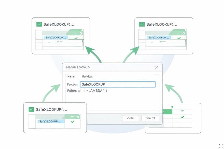
• Step 4: Save it as a Named Formula. Use Formulas > Name Manager, create a new name (e.g., SafeXLOOKUP), and paste the LAMBDA into “Refers to”.
• Step 5: Replace repeated XLOOKUPs with the named function. This standardizes behavior across sheets.

Example LAMBDA (as a formula you can paste to test):

=LAMBDA(v, keys, returns, missingText, LET(isBlank, v="", c, IF(isBlank, 0, COUNTIF(keys, v)), IF(isBlank, "", IF(c=0, missingText, IF(c>1, "DUPLICATE KEY", XLOOKUP(v, keys, returns, missingText))))))

Once saved as SafeXLOOKUP, usage becomes:

=SafeXLOOKUP([@CustomerID], Customers[CustomerID], Customers[Region], "MISSING")

From an audit perspective, this is powerful: reviewers can inspect the single definition of SafeXLOOKUP and know that all dependent columns follow the same rule.

Reusable SUMIFS with LAMBDA (standard criteria patterns)

SUMIFS often repeats the same criteria structure (site + SKU + date range + type). You can wrap this into a LAMBDA to reduce mistakes like swapping criteria ranges or forgetting a boundary.

Example: define a function QtyByType that sums quantity for a given SKU, site, type, and date range.

=LAMBDA(sku, site, t, d1, d2, LET(hasInputs, AND(sku<>"",site<>"",d1<>"",d2<>""), IF(NOT(hasInputs), "", SUMIFS(Transactions[Qty], Transactions[SKU], sku, Transactions[Site], site, Transactions[Type], t, Transactions[Date], ">="&d1, Transactions[Date], "<="&d2))))

After saving as QtyByType, you can compute components clearly:

=LET(receipts, QtyByType([@SKU],[@Site],"Receipt",[@MonthStart],[@MonthEnd]), issues, QtyByType([@SKU],[@Site],"Issue",[@MonthStart],[@MonthEnd]), receipts-issues)

This reads like an audit schedule: define receipts, define issues, compute net.

Putting it together: an audit-friendly metric pattern

Many operational dashboards rely on a small set of metrics repeated across dimensions (site, SKU, customer, week/month). A robust pattern is: (1) validate key uniqueness, (2) retrieve attributes with safe lookups, (3) aggregate transactions with standardized SUMIFS logic, (4) compute final KPIs with LET so each step is named.

Example: On-time rate by customer with explicit rules

Scenario: A Shipments table has ShipmentID, CustomerID, ShipDate, PromisedDate, DeliveredDate, Status. You want an on-time flag and then an on-time rate by customer for a period.

On-time flag (in Shipments):

=LET(del, [@DeliveredDate], prom, [@PromisedDate], st, [@Status], IF(OR(st<>"Delivered",del="",prom=""),"",IF(del<=prom,1,0)))

Audit-friendly: blanks indicate “not applicable / not measurable yet” rather than forcing 0.

On-time rate for a customer in a summary table (CustomerID in the row, MonthStart/MonthEnd in columns):

=LET(id, [@CustomerID], d1, [@MonthStart], d2, [@MonthEnd], onTime, SUMIFS(Shipments[OnTimeFlag],Shipments[CustomerID],id,Shipments[DeliveredDate],">="&d1,Shipments[DeliveredDate],"<="&d2), measured, COUNTIFS(Shipments[CustomerID],id,Shipments[DeliveredDate],">="&d1,Shipments[DeliveredDate],"<="&d2,Shipments[OnTimeFlag],">=0"), IF(measured=0,"",onTime/measured))

Notes for audit: measured counts only rows where the flag is numeric (0 or 1). This avoids counting undelivered shipments as late by default.

Common audit pitfalls and safer alternatives

Pitfall: using IFERROR to hide everything

IFERROR can be useful, but it can also hide real issues (like duplicates or wrong column references). Prefer targeted checks: ISNA for not-found, COUNTIF/COUNTIFS for duplicates, and explicit blank handling for incomplete inputs.

Less auditable:

=IFERROR(XLOOKUP(A2,Customers[CustomerID],Customers[Region]),"")

More auditable:

=LET(id,A2,c,COUNTIF(Customers[CustomerID],id),IF(id="","",IF(c=0,"MISSING",IF(c>1,"DUPLICATE",XLOOKUP(id,Customers[CustomerID],Customers[Region],"MISSING")))))

Pitfall: mixing text and numeric outputs in KPI cells

Returning text like “MISSING” in a numeric KPI cell can break charts and downstream calculations. A more audit-friendly approach is to keep numeric outputs numeric (or blank) and create a separate status/flag column for messages. If you must show messages, do it in a companion cell.

Pitfall: inconsistent criteria across SUMIFS copies

Copying SUMIFS across sheets often leads to subtle drift: one version uses ShipDate, another uses DeliveredDate; one includes Status, another doesn’t. Standardize with LAMBDA (or at least with LET naming) so the criteria are centralized and visible.

Pitfall: approximate matches in operational IDs

Approximate match lookups can silently return wrong results when IDs are not sorted or when new codes are inserted. For operational keys, default to exact match behavior and explicitly handle not-found cases.

Practical checklist: making a formula easy to audit

• Can you identify the key? The lookup value should be a single field (CustomerID, SKU, etc.).
• Are source columns explicit? Use Table[Column] references for lookup and aggregation ranges.
• Is missing data handled intentionally? Use if_not_found, ISNA, and blank short-circuits.
• Are duplicates surfaced? Use COUNTIF/COUNTIFS checks where keys must be unique.
• Are intermediate steps named? Use LET to label components like receipts, issues, unitPrice, measured.
• Is repeated logic standardized? Use LAMBDA Named Formulas for safe lookups and common SUMIFS patterns.
• Do numeric outputs stay numeric? Keep flags/messages separate from KPI values when possible.