Sample Size Intuition, Power, and Guardrail Metrics for Safe Rollouts

Why sample size and power matter in business experiments

Once you can run an experiment, the next practical question is: “How long do we run it, and how many users do we need?” Sample size and power are not academic details; they determine whether you can reliably detect effects that are large enough to matter, while also protecting the business from harmful rollouts. In practice, teams often fail in two ways: (1) running tests that are too small, producing noisy results and flip-flopping decisions, or (2) running tests far larger than needed, wasting time and opportunity cost. A good plan balances decision urgency, expected effect size, baseline variability, and safety constraints.

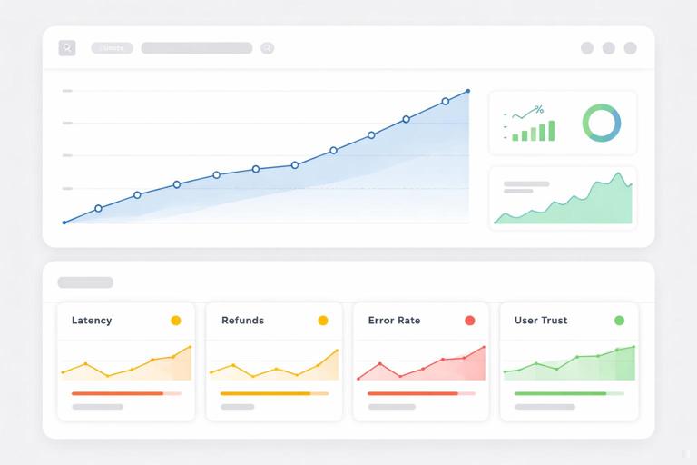
Power planning is also a communication tool. It forces alignment on what “meaningful impact” means (the minimum detectable effect), what risk of false negatives is acceptable (power), and what risk of false positives is acceptable (significance level). Guardrail metrics complement this by ensuring that even if the primary metric improves, you do not accidentally degrade critical aspects like reliability, refunds, or user trust.

Core intuition: signal, noise, and the minimum detectable effect (MDE)

Think of an experiment as trying to hear a signal (the true treatment effect) through noise (random variation in user behavior and measurement). Sample size increases your ability to separate signal from noise. The key quantity you must choose is the minimum detectable effect (MDE): the smallest effect you care to detect with high probability. If the true effect is smaller than the MDE, your test is not designed to reliably detect it, and “no significant difference” will be ambiguous.

Three levers determine how hard the problem is:

• Effect size (signal): Smaller expected changes require larger samples.
• Outcome variability (noise): More variable metrics require larger samples.
• Confidence requirements: Higher power and stricter significance thresholds require larger samples.

In business terms: if you want to detect a 0.2% lift in conversion with high confidence, you will need a lot of traffic. If you only need to detect a 5% lift, you can decide faster.

Continue in our app.

• Listen to the audio with the screen off.
• Earn a certificate upon completion.
• Over 5000 courses for you to explore!

Or continue reading below...

Download the app

Absolute vs relative effects

Be explicit about whether the MDE is absolute (e.g., “+0.3 percentage points conversion”) or relative (e.g., “+3% relative lift”). For a baseline conversion of 10%, a +3% relative lift equals +0.3 percentage points. Teams often mix these up and under- or over-estimate required sample size.

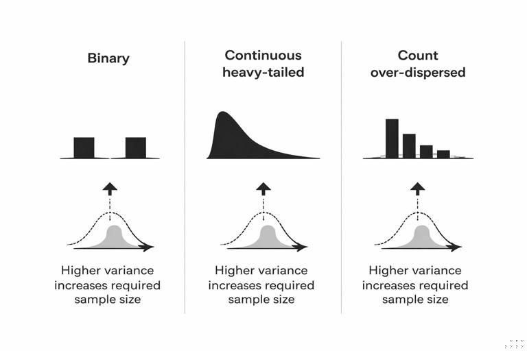
Why variance differs by metric type

Binary metrics (converted vs not) have variance driven by the baseline rate. Continuous metrics (revenue per user, time on site) can have heavy tails and large variance, inflating sample size. Count metrics (number of sessions) often have over-dispersion. This matters because sample size formulas depend on variance; two metrics with the same “business importance” can have wildly different statistical difficulty.

Power, Type I error, and Type II error in decision terms

Power analysis revolves around two kinds of mistakes:

• Type I error (false positive): You ship a change that doesn’t truly help (or might even hurt), because the experiment result looked positive by chance. The probability of this is controlled by the significance level, often denoted α (commonly 0.05).
• Type II error (false negative): You fail to ship a change that truly helps, because the experiment didn’t have enough sensitivity. The probability of this is β; power is 1 − β (commonly 0.8 or 0.9).

Translate these into business costs. A false positive might cause revenue loss, user churn, or operational risk. A false negative might mean missed growth. Different product areas should choose different thresholds. For example, a payments change might require stricter false-positive control and stronger guardrails than a minor UI tweak.

One-sided vs two-sided tests

Many business experiments are evaluated with two-sided tests (detect improvement or harm). A one-sided test can reduce required sample size, but only makes sense if you truly would not act on a negative result beyond “don’t ship.” In many organizations, detecting harm is itself a key outcome, so two-sided testing is safer and more aligned with guardrails.

Practical sample size intuition (without getting lost in formulas)

You can build strong intuition with a few rules of thumb:

• Halving the MDE roughly quadruples sample size. Detecting smaller effects is expensive.
• Higher baseline conversion can reduce variance up to a point, but not always enough to matter. Binary variance is p(1−p), which is highest near 50% and lower near 0% or 100%.
• Heavy-tailed metrics (like revenue) often need variance reduction techniques or longer tests. Otherwise, a few outliers dominate.
• More segments means more data. If you need reliable results by country, device, or new vs returning users, plan for it; subgroup analysis inflates uncertainty.

Also remember that sample size is not just “number of users.” It is the number of independent experimental units that contribute information. If you randomize by user but measure daily outcomes, repeated days from the same user are correlated; you do not get “free” sample size from repeated measurements unless your analysis accounts for it correctly.

Minimum run time and seasonality

Even if you have enough users quickly, you may need a minimum duration to cover day-of-week patterns, pay cycles, or marketing rhythms. A common practice is to run at least one full business cycle (often 1–2 weeks) to avoid bias from temporal patterns. This is not a substitute for sample size; it is an additional constraint.

Step-by-step: planning sample size and power for an online experiment

Step 1: Choose the primary metric and its unit

Define the primary metric in the same unit you will analyze (user-level conversion, revenue per user, etc.). Confirm logging completeness and metric definition consistency across variants. If the metric is rare (e.g., chargebacks), expect large sample requirements and consider whether a proxy metric is acceptable for short-term tests.

Step 2: Estimate baseline rate/mean and variance

Use recent historical data from the same population and time window. For a binary metric, baseline conversion p is enough. For continuous metrics, estimate mean and standard deviation (or use robust measures if outliers are extreme). If the metric distribution is highly skewed, consider transformations (e.g., log(1+x)) or winsorization policies—decide these before looking at experiment results.

Step 3: Set the MDE based on business value

Pick the smallest effect worth acting on. A practical way is to translate effect into dollars or strategic impact. Example: if a 0.2 percentage point lift in checkout conversion yields $200k/month, and engineering cost is $50k, then 0.2pp might be a reasonable MDE. If the change is risky, you might require a larger effect to justify rollout.

Step 4: Choose α and desired power

Typical defaults are α = 0.05 (two-sided) and power = 0.8. For high-risk areas, consider α = 0.01 and/or power = 0.9, recognizing that this increases required sample size. Align these choices with decision stakes and guardrail strictness.

Step 5: Compute required sample size (and convert to run time)

Use a power calculator appropriate to the metric type. For binary conversion, use a two-proportion test approximation; for continuous metrics, use a two-sample t-test approximation (or nonparametric/bootstrapped power if needed). Convert required sample size into duration using expected traffic and allocation (e.g., 50/50 split). Add a buffer for data loss, exclusions, and unexpected traffic dips.

Step 6: Predefine stopping rules and analysis plan

Decide whether you will run to a fixed sample size, use sequential testing, or use group sequential boundaries. Avoid “peeking” and stopping early based on noisy significance unless you use a method designed for it. Predefine how you will treat missing data, bots, internal traffic, and multiple comparisons across metrics.

Step 7: Validate with a back-of-the-envelope sanity check

Before launching, sanity-check the output: if the calculator says you need 50 million users to detect a tiny effect, that is plausible; it means your desired sensitivity is extremely high relative to noise. Decide whether to increase MDE, change metric, use variance reduction, or accept longer duration.

Worked example: conversion rate experiment

Suppose you are testing a new onboarding flow. Baseline activation rate is 12%. You care about at least a +0.6 percentage point absolute lift (to 12.6%), because that translates into meaningful downstream revenue. You choose α = 0.05 two-sided and power = 0.8.

Intuition: a 0.6pp lift on a 12% baseline is a 5% relative lift. That is moderate. If your site has 200k eligible new users per week and you split 50/50, you might expect to finish in a couple of weeks. If traffic is only 20k/week, you may need months, and you should revisit whether the MDE is realistic or whether you can use a more sensitive metric.

Even without exact numbers, you can anticipate tradeoffs: if you reduce MDE to +0.3pp, sample size will jump substantially (roughly 4×). If you insist on power 0.9, sample size increases again. This is why agreeing on MDE is often the most important step.

Variance reduction: getting more power without more users

If sample size requirements are too large, you can sometimes reduce variance rather than increase traffic. Common approaches include:

• Covariate adjustment (CUPED-style): Use pre-experiment behavior (e.g., prior week revenue) as a covariate to explain some outcome variance. This can materially reduce required sample size when pre-period metrics correlate with post-period outcomes.
• Stratification / blocking: Ensure balance across key segments (country, device) and analyze with stratified estimators to reduce variance.
• Ratio metrics handled carefully: Metrics like revenue/session can be noisy; sometimes analyzing numerator and denominator separately or using delta-method/Fieller approaches improves stability.
• Outlier policies: Predefined winsorization or robust estimators can reduce variance for heavy-tailed metrics, but must be justified and applied consistently.

Variance reduction is not “cheating.” It is a principled way to use information you already have to improve sensitivity, as long as it is planned in advance and does not introduce bias.

Guardrail metrics: designing for safe rollouts

A primary metric tells you whether the change achieves its main goal. Guardrail metrics ensure you do not pay for that improvement with unacceptable harm elsewhere. Guardrails are especially important when optimizing a narrow metric can create perverse incentives (e.g., increasing conversion by making cancellation harder).

Characteristics of good guardrails

• Directly tied to user or business safety: error rates, latency, refunds, customer support contacts, policy violations.
• Hard to game: metrics that reflect real outcomes rather than easily manipulated proxies.
• Fast feedback: ideally they move quickly enough to detect harm during the experiment window.
• Operationally actionable: if a guardrail trips, you know what to do (rollback, throttle, investigate).

Common guardrail categories

• Reliability and performance: crash rate, API error rate, p95 latency, timeouts.
• Trust and policy: complaint rate, abuse reports, fraud flags, chargebacks.
• Customer experience: unsubscribe rate, return rate, support tickets per user.
• Financial integrity: gross margin, discount leakage, refunds, promo abuse.

Guardrails should be chosen based on plausible failure modes of the change. For example, a new recommendation algorithm might improve click-through (primary) but increase content complaints (guardrail). A checkout change might improve conversion but increase payment failures or refunds.

How to set guardrail thresholds (and avoid “metric theater”)

A guardrail is only useful if it has a predefined threshold that triggers action. Otherwise, teams can rationalize away harm after the fact. Thresholds should reflect both statistical uncertainty and business tolerance.

Approach 1: Non-inferiority margins

For each guardrail, define a maximum acceptable degradation (a non-inferiority margin). Example: “p95 latency must not increase by more than 20ms” or “refund rate must not increase by more than 0.05 percentage points.” Then evaluate whether the experiment data rules out worse-than-margin harm with sufficient confidence.

Approach 2: Risk-based alerting bands

For operational metrics, you may use alerting bands: if the guardrail moves beyond a threshold (absolute or relative), pause or ramp down even before statistical certainty, because the cost of waiting is high. This is common for reliability metrics where harm can cascade.

Approach 3: Composite safety scorecards

Sometimes you need multiple guardrails. A scorecard approach defines “must-pass” metrics (hard stops) and “watch” metrics (require investigation). Keep the must-pass list short; too many hard stops can paralyze decision-making and inflate false alarms.

Power for guardrails: the hidden trap

Teams often power the experiment for the primary metric but forget that guardrails may be rarer or noisier. If a guardrail event is rare (e.g., chargebacks), your experiment may be underpowered to detect meaningful harm. This creates a false sense of safety: “No significant increase in chargebacks” might simply mean “we didn’t have enough data.”

Practical mitigations:

• Use leading indicators: If chargebacks are delayed, use earlier signals like payment failures or fraud scores as guardrails during rollout.
• Extend observation windows: Keep monitoring guardrails after ramp-up, especially for delayed outcomes like refunds.
• Use higher sensitivity for safety metrics: Consider stricter thresholds and lower tolerance for degradation, combined with operational monitoring.
• Plan separate power checks: For key guardrails, compute detectable harm given expected sample size and decide if that is acceptable.

Safe rollouts: combining experimentation with staged ramping

Even with a well-powered experiment, many organizations deploy changes gradually to manage risk. A safe rollout treats exposure as a controlled ramp: 1%, 5%, 25%, 50%, 100%, with checks at each stage. The experiment can be embedded within this ramp (e.g., holdout control) or run first at a fixed split and then ramp after decision.

Step-by-step: a practical safe rollout plan with guardrails

Step 1: Define ramp stages and decision gates

Example stages: 1% for 2 hours, 5% for 1 day, 25% for 2 days, 50% until sample size reached, then 100%. Each gate has criteria: primary metric trending acceptable and no guardrail breaches.

Step 2: Set real-time monitoring for must-pass guardrails

For early stages, prioritize fast operational metrics (errors, latency, crash rate). These should be monitored in near real time with automated alerts. Early-stage gates are about preventing catastrophic failures, not measuring long-term business impact.

Step 3: Use holdouts to preserve causal measurement during ramp

If you ramp to 100% without a persistent control group, you lose the ability to measure incremental impact cleanly. A common pattern is to keep a small holdout (e.g., 5–10%) on the old experience for a defined period, enabling continued measurement of primary and guardrail metrics while the business benefits from broad rollout.

Step 4: Decide what triggers rollback vs pause vs continue

Define actions for each guardrail outcome:

• Rollback: clear harm beyond threshold or severe operational issues.
• Pause and investigate: ambiguous movement, data quality concerns, or segment-specific anomalies.
• Continue ramp: metrics within bounds and data quality checks pass.

Step 5: Segment-aware safety checks

Overall averages can hide localized harm. For safety, check key segments where risk concentrates (e.g., a new payment method in one country, older devices, high-value customers). Predefine which segments are safety-critical to avoid post-hoc cherry-picking.

Multiple metrics and error control: keeping decisions coherent

When you evaluate one primary metric plus several guardrails, you face a tradeoff: if you treat every metric as a hypothesis test at α = 0.05, you increase the chance of false alarms. But if you ignore multiplicity entirely, you may overreact to noise.

Practical guidance:

• One primary metric drives the “ship for impact” decision. Keep it singular when possible.
• Guardrails are often asymmetric. You care more about detecting harm than detecting improvement. Consider one-sided harm checks or non-inferiority framing.
• Use a hierarchy. Primary metric tested formally; must-pass guardrails have predefined thresholds; watch metrics inform investigation rather than automatic blocking.

Implementation checklist: what to write down before launch

• Primary metric: definition, unit, aggregation, inclusion/exclusion rules.
• MDE: absolute and relative, and business rationale.
• α and power: and whether tests are one- or two-sided.
• Sample size and duration: required N per variant, expected run time, minimum duration constraint.
• Variance reduction plan: covariates, stratification, outlier handling (predefined).
• Guardrails: must-pass vs watch, thresholds/margins, monitoring cadence.
• Stopping rules: fixed-horizon vs sequential, and who can stop the test.
• Rollout plan: ramp stages, gates, rollback criteria, holdout strategy.
• Data quality checks: sample ratio mismatch checks, missingness, logging parity across variants.

Code sketch: power planning inputs and a simple calculator workflow

The exact computation depends on your tooling, but the workflow is consistent: gather baseline, choose MDE, choose α/power, compute N, convert to time, then validate guardrail detectability.

# Pseudocode workflow (language-agnostic) for a binary primary metric (conversion) 1) Inputs baseline_p = 0.12 alpha = 0.05 power = 0.80 mde_abs = 0.006   # +0.6 percentage points allocation = 0.50  # 50/50 split weekly_eligible_users = 200000 2) Compute required sample size per group n_per_group = power_calc_two_proportions(p1=baseline_p, p2=baseline_p + mde_abs, alpha=alpha, power=power, two_sided=True) 3) Convert to duration total_needed_users = 2 * n_per_group weeks_needed = total_needed_users / weekly_eligible_users 4) Guardrail detectability check (example: refund rate baseline 0.8%) guardrail_baseline = 0.008 guardrail_harm_margin = 0.0005 # +0.05pp unacceptable detectable_harm = detectable_diff_two_proportions(p1=guardrail_baseline, n=n_per_group, alpha=alpha, power=0.80) if detectable_harm > guardrail_harm_margin:     flag("Underpowered for refund guardrail; add leading indicator or extend monitoring")

This sketch highlights a key habit: treat guardrails as first-class citizens in planning. If you cannot detect meaningful harm in a rare guardrail, compensate with operational monitoring, longer observation, or alternative metrics.