Estimating Treatment Effects and Understanding Uncertainty

What it Means to “Estimate a Treatment Effect”

Once a causal question is identified and a study design is chosen, the next task is estimation: turning observed data into a numerical answer for “how much did the treatment change the outcome?” In practice, you rarely want only a single number; you also need to quantify uncertainty so decision-makers understand how stable that estimate is and what range of true effects is plausible.

Two core ideas guide this chapter:

• Estimands: the precise causal quantity you want to learn (for example, the average treatment effect for all eligible users, or only for those who actually complied).
• Estimators: the recipe (a formula or algorithm) that uses your data to produce an estimate of that estimand.

Keeping estimands and estimators separate prevents confusion. For example, “difference in means” is an estimator; “average treatment effect (ATE)” is an estimand. Many estimators can target the same estimand, and the same estimator can target different estimands depending on how you define the population and handle missingness, noncompliance, or clustering.

Common Treatment Effect Estimands Used in Business

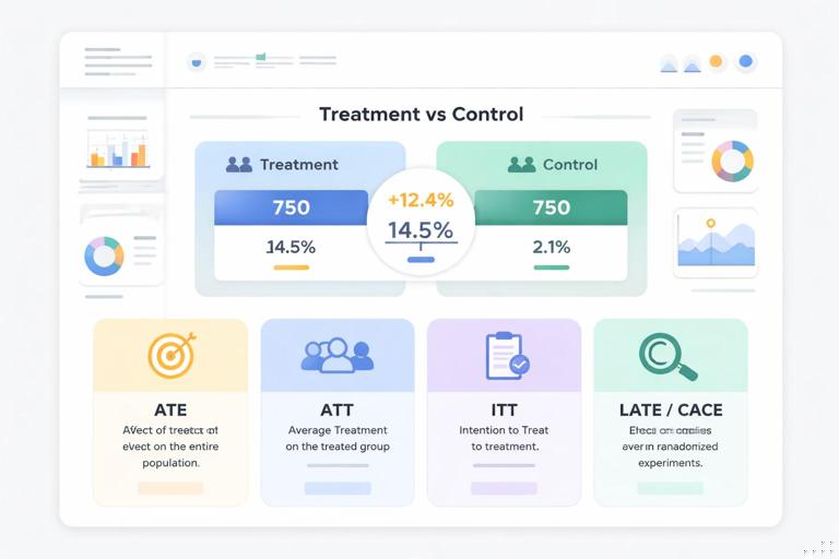
Average Treatment Effect (ATE)

ATE is the average causal effect if everyone in the target population were treated versus if everyone were untreated. It is often the default estimand when you can assign treatment and want a single number summarizing impact.

Example: “If all eligible customers saw the new checkout, how much would average revenue per visitor change compared with the old checkout?”

Continue in our app.

• Listen to the audio with the screen off.
• Earn a certificate upon completion.
• Over 5000 courses for you to explore!

Or continue reading below...

Download the app

Average Treatment Effect on the Treated (ATT)

ATT is the average effect among those who actually received treatment. This matters when treatment uptake is selective (for example, a feature is optional) and you want to understand the effect for adopters.

Example: “Among customers who enabled the new recommendation widget, how much did their purchase rate change?”

Intent-to-Treat (ITT)

ITT is the effect of assignment to treatment, regardless of whether the unit complied. ITT is often the most operationally relevant estimand when assignment is what you control (e.g., you can assign exposure, but cannot force engagement).

Example: “If we roll out the new onboarding flow to 50% of new users, how much does retention change, even if some users skip steps?”

Local Average Treatment Effect (LATE) / Complier Average Causal Effect (CACE)

LATE (also called CACE) is the effect for “compliers” in settings with noncompliance and an instrument (often assignment). It answers: “What is the effect among those who take treatment if and only if assigned?”

Example: “Among users who would use the new feature only when it is enabled for them, what is the effect on engagement?”

Heterogeneous Treatment Effects (HTE)

Often you need effects by segment: new vs. returning customers, small vs. large accounts, different geographies, etc. These are conditional average treatment effects (CATE). Estimating HTE responsibly requires careful uncertainty handling and multiple-comparison discipline (discussed below).

Point Estimates: Turning Data into an Effect Size

A point estimate is a single best guess of the treatment effect given your data and estimator. The simplest case is a randomized experiment with a continuous outcome:

ATE_hat = mean(Y | T=1) - mean(Y | T=0)

For binary outcomes (conversion), the same difference-in-means estimator works on proportions. For ratio metrics (e.g., revenue per user), you may use a delta-method approximation, a ratio estimator, or a regression approach; the key is to ensure the estimator matches the estimand and that uncertainty is computed correctly for the metric type.

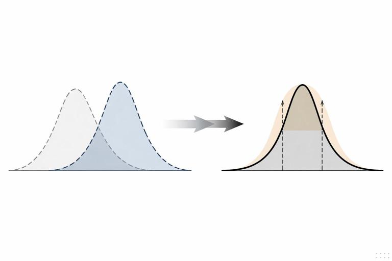
Regression as an Estimator (Not a Causal Assumption by Itself)

Linear regression is often used to estimate treatment effects because it can improve precision and adjust for covariates. In a randomized setting, adding pre-treatment covariates can reduce variance without changing the estimand.

Y = alpha + tau * T + beta'X + error

Here, tau estimates the treatment effect (for the chosen estimand and population). The practical benefit is narrower uncertainty intervals when X explains outcome variation.

For non-linear outcomes (binary, counts), generalized linear models can be used, but interpretability matters: the coefficient may be on a log-odds or log scale. If stakeholders need an effect in probability points or absolute counts, compute marginal effects and their uncertainty rather than reporting raw coefficients.

Uncertainty: Why a Single Number Is Not Enough

Every estimate is noisy because you observe a finite sample and outcomes vary. Uncertainty quantification answers: “If we repeated this study many times under the same conditions, how much would our estimate vary?”

Three practical uncertainty objects are used most often:

• Standard error (SE): typical variability of the estimator.
• Confidence interval (CI): a range of plausible values for the true effect under repeated sampling logic (frequentist).
• Credible interval: a range that contains the true effect with a stated probability under a Bayesian model.

Even if your organization prefers p-values, it is usually more decision-useful to communicate uncertainty as an interval around an effect size, plus the implied business impact range.

Interpreting a 95% Confidence Interval Correctly

A 95% CI does not mean “there is a 95% chance the true effect lies in this interval” (that is Bayesian language). It means: if you repeated the same procedure many times, 95% of the constructed intervals would contain the true effect.

Decision framing: treat the CI as a practical range of effects consistent with the data and assumptions. If the entire interval is above a business threshold (e.g., +0.5% conversion), you have stronger evidence to ship. If it straddles the threshold, you may need more data, a different design, or a different decision rule.

Step-by-Step: Estimating an Effect and Its Uncertainty (Difference in Means)

This workflow applies to many A/B tests and can be adapted to observational estimators as well.

Step 1: Define the estimand and analysis population

• Choose ATE vs. ITT vs. ATT (be explicit).
• Define inclusion/exclusion rules (e.g., eligible users, time window).
• Define the outcome metric precisely (e.g., 7-day retention, revenue per session).

Step 2: Compute group summaries

• Compute n1, mean1, var1 for treatment group.
• Compute n0, mean0, var0 for control group.

Step 3: Compute the point estimate

tau_hat = mean1 - mean0

Step 4: Compute the standard error

For independent units and unequal variances (common), use the Welch-style standard error:

SE(tau_hat) = sqrt( var1/n1 + var0/n0 )

Step 5: Construct a confidence interval

Approximate 95% CI (large samples):

CI_95 = tau_hat ± 1.96 * SE(tau_hat)

If sample sizes are small or distributions are heavy-tailed, prefer a t-based interval or bootstrap (below).

Step 6: Translate into business impact

Convert the effect into units stakeholders care about. Example: if tau_hat is +0.3 percentage points conversion and you have 2 million monthly visitors, the expected incremental conversions are roughly 0.003 × 2,000,000 = 6,000 per month. Apply the CI bounds to get a plausible range (e.g., 2,000 to 10,000).

Bootstrap Uncertainty: A Practical Tool for Complex Metrics

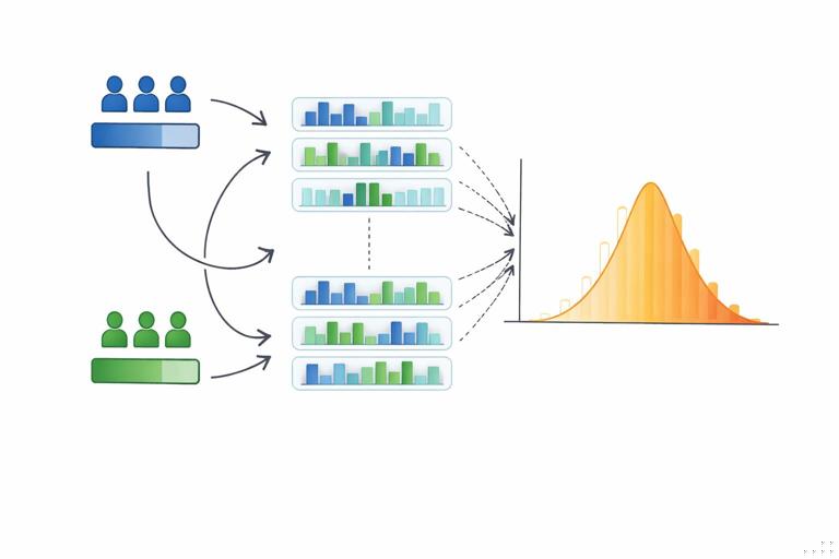
Many business metrics are not simple averages: medians, percentiles, ratios, revenue per active user, time-to-event summaries, or metrics with winsorization/capping. Analytical standard errors can be messy. The bootstrap is a general approach:

• Resample units with replacement within each group.
• Recompute the metric and the treatment effect for each resample.
• Use the distribution of bootstrap effects to estimate SEs and intervals.

Step-by-Step Bootstrap for a Ratio Metric

Suppose the metric is revenue per user (RPU) = total revenue / number of users, and you want the difference in RPU between treatment and control.

• Step 1: For b = 1…B (e.g., 2,000): resample users with replacement from treatment users; compute RPU_treat(b).
• Step 2: Resample users with replacement from control users; compute RPU_ctrl(b).
• Step 3: Compute effect(b) = RPU_treat(b) − RPU_ctrl(b).
• Step 4: Use the 2.5th and 97.5th percentiles of effect(b) as a 95% bootstrap percentile interval (or use BCa for better accuracy).

Bootstrap intervals are intuitive and often robust, but they rely on the sample being representative of the population and on independence assumptions at the resampling unit (see clustering below).

Clustering and Dependence: Getting Uncertainty Right When Observations Aren’t Independent

In many business settings, outcomes are correlated:

• Multiple sessions per user (within-user correlation).
• Users within the same account (B2B accounts).
• Geographic clusters, stores, or sales territories.
• Time dependence (daily metrics with autocorrelation).

If you ignore dependence and treat each row as independent, standard errors can be severely underestimated, producing overly narrow intervals and false confidence.

Practical fixes

• Aggregate to the randomization unit: If randomization is at user level, compute one outcome per user (e.g., total 7-day revenue per user) and analyze at user level.
• Cluster-robust standard errors: If you must use multiple observations per unit, use cluster-robust SEs at the unit level (user, account, store).
• Cluster bootstrap: Resample clusters (e.g., users) rather than individual rows.

Rule of thumb: uncertainty calculations should respect the unit at which treatment is assigned and the unit at which outcomes are correlated.

Noncompliance and “Dilution”: Estimating Effects When Not Everyone Takes the Treatment

Even with controlled assignment, real systems have noncompliance: users may not see the feature due to caching, app version, eligibility rules, or they may choose not to engage. This creates a gap between assignment and actual exposure.

ITT vs. per-protocol vs. LATE (practical guidance)

• ITT is usually the safest primary estimate because it preserves the comparability created by assignment and reflects real-world rollout impact.
• Per-protocol (analyzing only those who complied) can be biased because compliance is often related to user intent or ability.
• LATE/CACE can be estimated using assignment as an instrument when assumptions hold, yielding an effect among compliers. This is useful for understanding “true feature effect” among those who actually receive it, but it is not always the rollout effect.

A common operational pattern is to report both: ITT for decision-making about shipping, and an additional compliance-adjusted estimate for product understanding.

Multiple Metrics and Multiple Comparisons: Avoiding Overconfident Findings

Teams often track many outcomes: conversion, revenue, retention, engagement, support tickets, latency, etc. If you look at enough metrics, some will appear “significant” by chance. This is not a reason to ignore secondary metrics; it is a reason to manage uncertainty transparently.

Practical approaches

• Pre-specify a primary metric for the main decision and treat others as supporting evidence.
• Control false discoveries when scanning many segments or metrics (e.g., Benjamini–Hochberg false discovery rate control).
• Use hierarchical thinking: start with overall effect, then drill into segments with clear hypotheses and adjusted uncertainty.

When presenting results, distinguish between “decision-driving” estimates and exploratory findings, and show intervals rather than only p-values.

Heterogeneous Effects: Estimating Segment Impacts Without Fooling Yourself

Segment-level effects are valuable for targeting and risk management, but they are also noisy. Two common failure modes are (1) over-interpreting random variation and (2) choosing segments after seeing the data.

Step-by-step: a disciplined segment analysis

• Step 1: Choose segments based on business logic (e.g., new vs. returning, small vs. enterprise) before looking at results.
• Step 2: Estimate effects within each segment using the same estimator as overall.
• Step 3: Report uncertainty per segment (CIs) and consider multiplicity adjustments if many segments are tested.
• Step 4: Test for interaction: instead of comparing “significant vs. not significant,” estimate an interaction term (e.g., treatment × segment) and its interval.
• Step 5: Validate stability using holdout periods, repeated experiments, or shrinkage/partial pooling models when appropriate.

For many segments, consider models that partially pool estimates (e.g., hierarchical Bayesian models) to reduce extreme noise-driven segment effects.

Bayesian Uncertainty: Credible Intervals and Decision-Ready Probabilities

Bayesian analysis treats the treatment effect as uncertain and updates beliefs using data. The output is a posterior distribution for the effect, from which you can compute:

• Credible intervals (e.g., 95% posterior interval).
• Probability of beating a threshold (e.g., P(effect > 0)).
• Probability of meeting a business minimum (e.g., P(effect > +0.2% conversion)).

This is often easier to align with decisions: “There is an 88% probability the feature increases revenue” or “There is a 62% probability it exceeds the minimum viable lift.” The tradeoff is that results depend on modeling choices and priors; in business settings, use weakly informative priors unless you have strong, defensible prior knowledge.

Practical example: threshold-based decision

Suppose the minimum lift worth shipping is +$0.05 revenue per user. A Bayesian workflow can directly compute P(effect > 0.05). You can then define a rule such as: ship if P(effect > 0.05) > 0.9 and P(effect < 0) < 0.05, otherwise iterate or collect more data.

Sequential Monitoring and “Peeking”: Preserving Valid Uncertainty When Checking Results Over Time

Teams naturally want to check experiment results daily. But repeatedly testing and stopping when results look good inflates false positives if you use fixed-horizon p-values and intervals without adjustment.

Two practical ways to handle this:

• Group sequential methods: pre-plan a few interim looks (e.g., after 25%, 50%, 75%, 100% of sample) with adjusted boundaries so overall error rates remain controlled.
• Always-valid (time-uniform) inference: use methods that maintain validity under continuous monitoring, producing intervals or tests that remain correct no matter when you stop.

If your organization frequently “peeks,” adopting an always-valid approach or a pre-registered sequential plan prevents overconfident decisions based on early noise.

From Statistical Uncertainty to Decision Uncertainty

Even with a well-estimated effect and a clean interval, decisions depend on business context:

• Asymmetric costs: shipping a harmful change may be worse than delaying a beneficial one.
• Risk tolerance: some products require high confidence before changes (payments, trust & safety), others can iterate faster.
• Nonlinear value: a small lift may be valuable at scale, while a moderate lift may not justify engineering cost.

A practical way to connect uncertainty to action is to define a decision threshold (minimum effect worth acting on) and evaluate whether your uncertainty interval lies above it, overlaps it, or lies below it. When the interval overlaps the threshold, the next step is not “argue about significance,” but “choose whether to reduce uncertainty (more data, better measurement) or change the decision framing (targeting, staged rollout, alternative metric).”

Implementation Checklist: Estimation and Uncertainty in Practice

• State the estimand (ATE/ITT/ATT/LATE) and the analysis population.
• Use an estimator aligned to the metric (difference in means, regression adjustment, bootstrap for complex metrics).
• Compute uncertainty correctly (SE/CI or posterior intervals), respecting clustering and the randomization unit.
• Report effect sizes with intervals, not only p-values.
• Translate to business impact ranges using the interval bounds.
• Handle multiplicity when scanning many metrics/segments.
• Plan for monitoring (sequential or always-valid) if results will be checked repeatedly.