What Regression Discontinuity (RD) Is and When It Fits
Regression Discontinuity (RD) is a causal estimation approach designed for situations where a decision rule assigns treatment based on whether an observed “running variable” crosses a known threshold. Typical business examples include eligibility cutoffs (credit score ≥ 680), tier assignment (spend last 90 days ≥ $500), operational routing (distance to warehouse ≤ 20 miles), or compliance triggers (risk score ≥ 0.8). The key idea is that units just below and just above the cutoff are often very similar in all relevant ways except for treatment assignment, so the jump (discontinuity) in outcomes at the threshold can be interpreted as the causal effect of treatment for those near the cutoff.
RD is especially useful when you cannot randomize but you do have a deterministic or near-deterministic rule that creates a sharp change in treatment probability at a cutoff. Instead of comparing treated vs. untreated across the whole population (which can be heavily biased), RD focuses on a narrow neighborhood around the threshold where comparability is most plausible.
Core ingredients
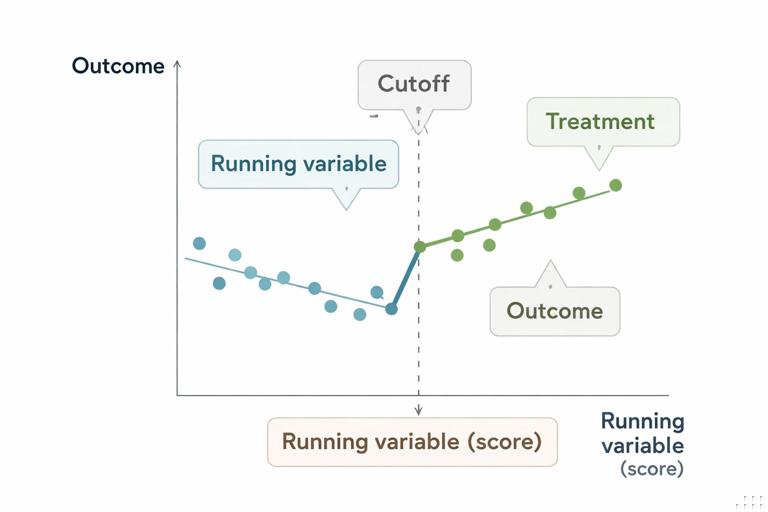
- Running variable (score): a continuous or ordinal measure used in the rule (credit score, risk score, revenue, age, test score).
- Cutoff: the threshold value that changes treatment assignment (e.g., 680).
- Treatment: the action triggered by the rule (approve loan, offer discount, assign case manager, expedite shipping).
- Outcome: the metric you care about (default rate, retention, profit, time-to-resolution).
RD estimates a local causal effect: the effect for units near the cutoff. This is often exactly what decision-makers need, because policy debates frequently revolve around “should we move the cutoff?” or “is the rule beneficial for borderline cases?”
Sharp vs. Fuzzy RD: Know Which World You’re In
Sharp RD
In sharp RD, treatment assignment is perfectly determined by the cutoff: everyone with score ≥ c is treated, and everyone with score < c is not. Example: an automated system that always grants free shipping to customers whose cart value is at least $50, with no exceptions.
Fuzzy RD
In fuzzy RD, the cutoff changes the probability of treatment, but not perfectly. This happens when humans override the rule, when there are capacity constraints, or when the rule is “guideline-like.” Example: a bank guideline says “approve if score ≥ 680,” but underwriters sometimes approve at 675 or deny at 690 due to additional information.
- Listen to the audio with the screen off.
- Earn a certificate upon completion.
- Over 5000 courses for you to explore!

Download the app
Fuzzy RD is common in real operations. It is not a deal-breaker; it changes the estimator. Instead of interpreting the outcome jump as the treatment effect directly, you treat the cutoff as an instrument that shifts treatment probability and estimate a local effect for “compliers” near the threshold.
Intuition: Why the Cutoff Creates a Quasi-Experiment
Imagine two customers with risk scores 679.9 and 680.1. If the score is measured precisely and the cutoff is enforced, these customers are nearly identical in risk. If one gets the intervention and the other does not, the difference in outcomes can be attributed to the intervention rather than underlying differences—provided that nothing else changes discontinuously at 680.
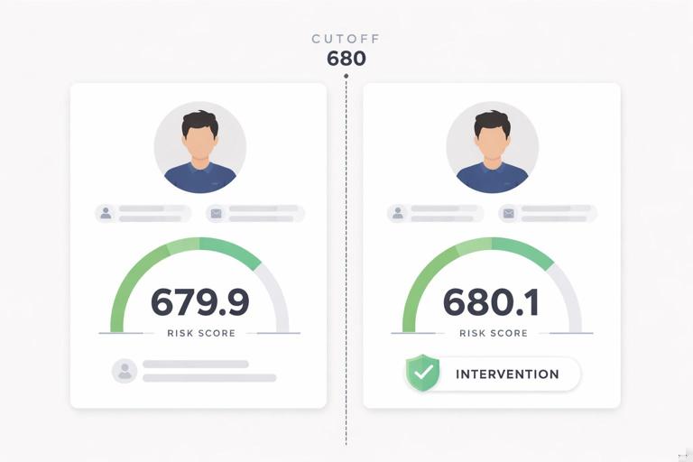
RD relies on a continuity idea: absent treatment, the expected outcome would change smoothly with the running variable. The cutoff introduces a discrete jump in treatment assignment, so any discrete jump in outcomes at that exact point is attributed to treatment.
Step-by-Step: Implementing RD in a Business Setting
Step 1: Write down the assignment rule and confirm the cutoff is real
Document the operational rule: what variable is used, how it is computed, when it is computed, and what cutoff is applied. Confirm that the cutoff is not changing over time or applied differently across teams. If there are multiple cutoffs (tiers), start with one cutoff and treat others carefully (you can analyze each threshold separately).
Example: “Customers with a churn risk score ≥ 0.70 are assigned to the retention outreach team within 24 hours.”
Step 2: Define the estimand you want (and accept it’s local)
RD answers: “What is the causal effect of treatment for units at (or very near) the cutoff?” This is a local average treatment effect around the threshold. If you need the effect for the entire population, RD alone won’t give it without additional assumptions. However, RD is excellent for decisions like adjusting the cutoff, evaluating whether the rule helps borderline cases, or validating that the intervention is beneficial where it is actually being applied.
Step 3: Assemble data with the right timestamps
RD is sensitive to timing. You need the running variable measured before treatment assignment and outcomes measured after. Also capture whether treatment actually occurred (especially for fuzzy RD), and any covariates you may use for diagnostics.
- Running variable value and timestamp (e.g., risk score at 9am Monday)
- Cutoff value and version of the scoring model
- Treatment indicator and timestamp (e.g., outreach call logged)
- Outcome window definition (e.g., churn within 30 days)
- Key covariates for balance checks (tenure, plan type, region)
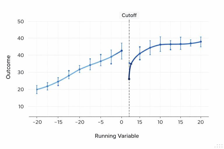
Step 4: Visualize the discontinuity
Before fitting models, plot the outcome against the running variable with a vertical line at the cutoff. Use binned averages (e.g., bins of width 0.01 for a 0–1 score, or 5 points for a credit score) and overlay a smooth fit on each side. This is not just for storytelling; it helps detect obvious issues like nonlinearity, outliers, or other discontinuities.
Also plot the treatment rate against the running variable. In sharp RD, you should see a near-step function from 0 to 1 at the cutoff. In fuzzy RD, you should see a clear jump in treatment probability at the cutoff.
Step 5: Choose a bandwidth (how close to the cutoff?)
The bandwidth determines which observations are considered “near enough” to be comparable. Too wide and you include units that differ meaningfully; too narrow and you lose precision. In practice, you can use data-driven bandwidth selection methods, but you should still sanity-check whether the chosen window makes business sense.
A practical workflow:
- Start with a moderate bandwidth (e.g., ±0.05 around a 0–1 score cutoff, or ±20 points around a credit score cutoff).
- Estimate the effect.
- Repeat with narrower and wider bandwidths to see if results are stable.
- Prefer specifications that are stable and not overly sensitive.
Step 6: Fit a local model on each side of the cutoff
RD is usually implemented with local linear regression: fit a line to the outcome vs. running variable on the left of the cutoff and another line on the right, using only observations within the bandwidth. The estimated treatment effect is the difference between the two fitted lines at the cutoff.
Why local linear? It tends to behave well near boundaries and avoids overfitting that can create artificial wiggles. Higher-order polynomials can look impressive but can be unstable and misleading near the cutoff.
Sharp RD model (conceptually): outcome = intercept + slope_left*(score-c) + treatment*(jump at cutoff) + slope_change*(score-c)*treatment + error.
Fuzzy RD model (conceptually): use the cutoff indicator as an instrument for treatment: first estimate the jump in treatment probability at the cutoff, then scale the outcome jump by that treatment jump.
Step 7: Compute robust uncertainty
Because RD focuses on a narrow region and uses nonstandard weighting, use robust standard errors appropriate for RD (many statistical packages implement this). If your data has clustering (e.g., by store, agent, region), cluster standard errors accordingly, because outcomes may be correlated within clusters.
Step 8: Run RD validity diagnostics (non-negotiable)
RD can be very credible when its assumptions hold, and very misleading when they don’t. Diagnostics are how you earn trust.
Key Assumptions and How to Check Them in Practice
1) No precise manipulation of the running variable around the cutoff
If people can “game” the score to barely qualify, then units just above and below may not be comparable. Examples: sales reps adjusting reported income to push a customer over a threshold, or customers timing purchases to hit a tier.
How to check:
- Density test: look for a spike in the distribution of the running variable just above the cutoff (a “bunching” pattern).
- Operational audit: review whether the score is computed from immutable data (e.g., third-party bureau score) vs. editable fields.
- Heaping: check for suspicious rounding (e.g., many values exactly at 680 or 700).
2) Continuity of potential outcomes and covariates at the cutoff
Absent treatment, the outcome should evolve smoothly with the running variable. A practical implication: other variables should not jump at the cutoff unless the treatment causes them to.
How to check:
- Covariate balance: plot and test whether pre-treatment covariates (tenure, baseline spend, region mix) show discontinuities at the cutoff.
- Placebo outcomes: use outcomes measured before treatment (e.g., prior-month churn, prior-week spend) and verify no jump at the cutoff.
- Multiple cutoffs: if you have other thresholds, verify that the jump is specific to the policy cutoff you’re studying.
3) No other policy changes at the same cutoff
If crossing the threshold triggers multiple actions (e.g., outreach plus a discount plus priority support), the RD estimate captures the combined effect of the bundle. That may be acceptable, but be explicit: you are estimating the effect of the policy package, not a single component.
How to check: map all downstream actions tied to the cutoff and verify what changes at that point. If multiple actions change, consider whether you can isolate one (often you cannot) and adjust the question accordingly.
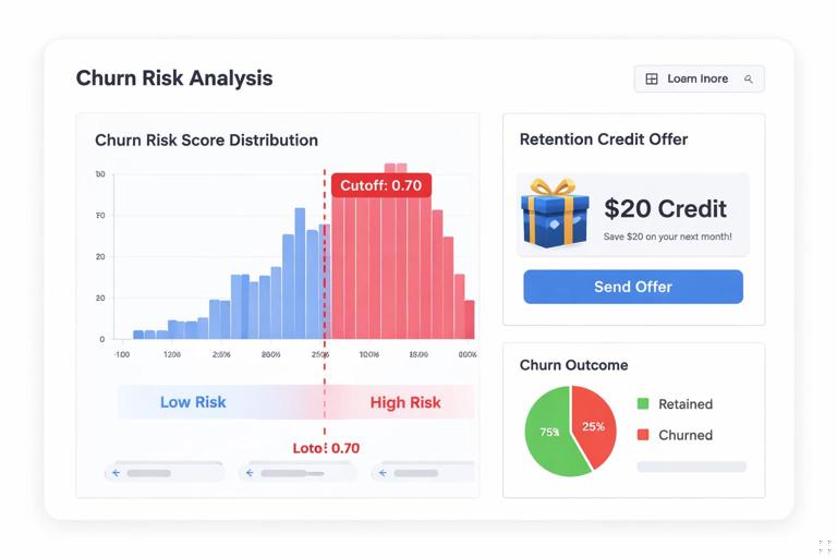
Practical Example 1: Eligibility Cutoff for a Retention Offer
Scenario: A subscription business offers a $20 retention credit to customers with churn risk score ≥ 0.70. You want to know whether the credit reduces churn for borderline customers and whether the cutoff should be moved.
Implementation outline
- Running variable: churn risk score (0–1).
- Cutoff: 0.70.
- Treatment: credit offered (and ideally credit redeemed, but the policy is the offer).
- Outcome: churn within 30 days; also consider net revenue impact.
Sharp vs fuzzy: If the offer is automatically triggered, it’s closer to sharp RD. If agents sometimes skip the offer or offer it below 0.70, it’s fuzzy RD.
What you would do
- Plot treatment rate vs. score to confirm a jump at 0.70.
- Plot churn rate vs. score to see if there is a visible drop at 0.70.
- Estimate local linear RD within a bandwidth, say ±0.05 (scores 0.65–0.75), then test sensitivity to ±0.03 and ±0.07.
- Run covariate continuity checks: tenure, plan type, baseline usage should not jump at 0.70.
- Run a placebo test: churn in the 30 days before the score was computed should not jump at 0.70.
Decision use: If the RD estimate shows a meaningful churn reduction with acceptable margin impact near 0.70, you can justify keeping or expanding the policy. If the effect is near zero, you might raise the cutoff or redesign the intervention for borderline customers.
Practical Example 2: Credit Policy with Human Overrides (Fuzzy RD)
Scenario: A lender guideline says approve if credit score ≥ 680. Underwriters can override. You want the causal effect of approval on default risk for borderline applicants.

Here, treatment is “loan approved.” The cutoff affects approval probability but not deterministically, so this is fuzzy RD.
What fuzzy RD estimates in this context
Fuzzy RD estimates the effect of approval for applicants whose approval status is influenced by being just above vs. just below 680 (the “compliers” near the cutoff). This is often the most policy-relevant group: borderline applicants.
Operational checks that matter
- Confirm the score used at decision time is the same score stored in data (avoid post-decision recalculations).
- Check for manipulation: are there manual edits to inputs that feed the score?
- Ensure no other underwriting rules change at 680 (e.g., documentation requirements, pricing APR changes). If pricing changes too, the estimate reflects a bundle: approval plus pricing regime.
Design Choices That Commonly Make or Break RD
Bandwidth and functional form
Prefer local linear models with a principled bandwidth and sensitivity checks. Avoid high-degree polynomials across a wide range; they can create artificial curvature and exaggerate or hide discontinuities.
Don’t “control away” the running variable incorrectly
RD already conditions on the running variable by design. You can include additional covariates to improve precision, but you should not include variables that are affected by treatment (post-treatment variables), and you should not use covariates to justify a too-wide bandwidth. Covariates are for precision and diagnostics, not for making incomparable observations comparable.
Multiple cutoffs and tiered policies
Many businesses have tiering: e.g., score ≥ 0.70 gets offer A, ≥ 0.85 gets offer A+B. You can run RD at each cutoff, but interpret each estimate as the incremental effect of crossing that specific threshold (which may represent an incremental bundle). Be careful that the neighborhood around one cutoff does not overlap another cutoff’s treatment regime in a way that confuses interpretation.
Discrete running variables
If the running variable takes only a small number of values (e.g., integer scores with few unique points), RD becomes harder because “near the cutoff” may still mean large jumps in underlying risk. You can still proceed, but you must be more cautious: use appropriate methods for discrete running variables, ensure enough mass on both sides, and interpret results with more uncertainty.
Sorting and operational capacity constraints
Sometimes the cutoff is used to prioritize work, but capacity limits mean not everyone above the cutoff is treated. This creates fuzzy RD. Additionally, if capacity constraints vary by day, you can see treatment probability shift around the cutoff over time. In that case, consider estimating RD separately by period or including time controls, and verify that the discontinuity in treatment remains stable.
Interpreting RD Results for Business Decisions
Local effect and cutoff policy
RD tells you the effect for borderline units. This is directly actionable for cutoff tuning. For example, if the retention credit helps at 0.70, you might test expanding eligibility slightly downward. If it harms margin without reducing churn, you might tighten eligibility.
From effect to ROI near the threshold
Many RD outcomes are intermediate (conversion, churn). For decision-making, translate the local effect into dollars:
- Estimate incremental retained customers near the cutoff.
- Multiply by expected contribution margin per retained customer (within the relevant horizon).
- Subtract the cost of treatment (discount, agent time, operational cost).
Because RD is local, do this ROI calculation for the population mass near the cutoff (how many customers fall within the band you consider for policy changes), not for the entire customer base.
Heterogeneity around the cutoff
Even within a narrow band, effects can differ by segment (e.g., new vs. tenured customers). You can explore heterogeneity by estimating RD separately within segments, but keep sample size limitations in mind. A practical approach is to predefine a small number of segments that are operationally meaningful and large enough to support stable estimates.
Common Failure Modes and How to Avoid Them
Failure mode: The running variable is measured with error or changes after the decision
If the stored score is recomputed later using updated data, the “score at decision time” is not what you think it is. This can blur the discontinuity and bias estimates.
Fix: store immutable snapshots of the running variable at decision time, including model version and feature timestamping.
Failure mode: People manipulate the score near the cutoff
Gaming breaks comparability. You may still learn something (e.g., the effect of a policy plus gaming behavior), but it is not the clean causal effect you intended.
Fix: use a harder-to-manipulate running variable, tighten governance, or move to a design where assignment is less gameable (e.g., randomized audits around the cutoff, if allowed).
Failure mode: Another change happens at the same cutoff
If crossing the threshold changes both eligibility and pricing, the RD estimate is the combined effect. If you interpret it as “eligibility effect,” you will mislead stakeholders.
Fix: map the policy bundle; if needed, redesign operations so only one lever changes at a time, or accept the bundle estimand explicitly.
Failure mode: Using too-wide a window and extrapolating
RD is not a global model. If you estimate within ±0.20 and then claim the effect applies to all customers, you are overreaching.
Fix: keep the interpretation local; if you need broader generalization, treat RD as one input and combine with other evidence (e.g., targeted experiments or additional quasi-experimental analyses) rather than stretching RD beyond its support.
Minimal Pseudocode Workflow (Conceptual)
# Inputs: data with columns: score, treated, outcome, cutoff c, bandwidth h# 1) Keep observations near cutoffsubset = data[ abs(data.score - c) <= h ]# 2) Create centered running variablex = subset.score - c# 3) Fit local linear regression with separate slopes on each side# outcome ~ a + b*x + tau*I(score>=c) + d*x*I(score>=c)# tau is the RD estimate at the cutoff# 4) For fuzzy RD:# First stage: treated ~ a1 + b1*x + pi*I(score>=c) + d1*x*I(score>=c)# Reduced form: outcome ~ a2 + b2*x + rho*I(score>=c) + d2*x*I(score>=c)# LATE near cutoff = rho / pi# 5) Diagnostics:# - plot outcome vs score with bins# - plot treated vs score# - check covariate continuity# - density test around cutoff# 6) Sensitivity:# - repeat for multiple bandwidths and compare tau