When Instrumental Variables Are the Right Tool
Instrumental Variables (IV) methods are designed for situations where you cannot credibly remove confounding with the data you have, or where the treatment you want to evaluate is not perfectly followed (imperfect compliance). In business terms, IV is useful when the “thing you can assign or influence” is not the same as the “thing that actually happens,” and the actual thing is correlated with unobserved factors that also affect outcomes.
Two common patterns:
- Hidden confounding: You suspect an unmeasured variable drives both treatment uptake and outcomes (e.g., motivation, risk tolerance, urgency, manager quality).
- Imperfect compliance: You can randomize or quasi-randomize an encouragement or eligibility, but customers/employees don’t always comply (e.g., invited to a new feature but not all adopt; assigned to training but not all attend).
IV reframes the problem: instead of comparing people who took the treatment versus those who didn’t (which may be confounded), you compare groups based on an “instrument” that shifts treatment probability in a way that is as-good-as random and affects the outcome only through the treatment.
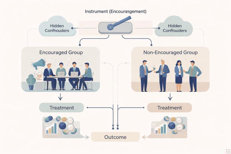
The Core Idea: An Instrument Creates Exogenous Variation in Treatment
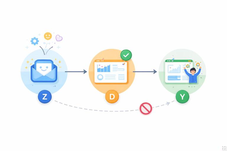
An instrument is a variable Z that changes the likelihood of receiving treatment D, and lets you isolate the part of D that is not entangled with hidden confounders. The outcome is Y.
Think of Z as a lever you can pull that nudges treatment up or down, while being otherwise unrelated to the outcome drivers.
- Listen to the audio with the screen off.
- Earn a certificate upon completion.
- Over 5000 courses for you to explore!

Download the app
Example 1: Encouragement Design for Feature Adoption
You want the causal effect of using a new dashboard (D) on weekly productivity (Y). People who choose to use the dashboard are likely more motivated, so comparing users vs non-users is biased. But you can randomize an encouragement email (Z) that increases adoption. The email itself should not affect productivity except by increasing dashboard use (no “direct effect”). Then Z can serve as an instrument for D.
Example 2: Operational Capacity as an Instrument (Quasi-Random)
Suppose you want the effect of a premium support call (D) on churn (Y). Calls are prioritized to customers who seem at risk (hidden confounding). However, call assignment is also influenced by random-ish agent availability at the time the ticket arrives (Z). If availability affects whether a call happens but does not directly affect churn except through the call, availability can be used as an instrument.
IV Assumptions in Business Language
IV works only if the instrument meets key assumptions. These are not just technicalities; they are the entire credibility of the estimate.
1) Relevance: The Instrument Must Move Treatment
Z must meaningfully change the probability or intensity of treatment D. If the encouragement email barely changes adoption, the instrument is weak and estimates become noisy and potentially biased.
Practical check: in the first-stage model (D on Z and controls), Z should have a strong effect. A common rule of thumb in linear settings is a first-stage F-statistic above ~10, but you should also look at the actual lift in treatment probability and whether it is stable across segments.
2) Independence (As-Good-As Random): Z Is Not Confounded With Y
Z should be unrelated to unobserved factors that affect Y. Random assignment of Z is the cleanest way to satisfy this. If Z is “agent availability,” you must argue that availability is not systematically correlated with customer type, ticket severity, or time-of-day patterns that also affect churn (or you must control for those patterns convincingly).
3) Exclusion Restriction: Z Affects Y Only Through D
This is often the hardest. The encouragement email must not directly change productivity by, say, reminding people to work harder, or by providing tips unrelated to the dashboard. Similarly, agent availability must not change customer satisfaction directly (e.g., shorter wait times) unless that shorter wait time is part of the “treatment” you intend to measure.
In practice, you strengthen exclusion by designing Z to be as “mechanical” as possible: a nudge that only changes access/uptake, not other channels.
4) Monotonicity (No Defiers): The Instrument Doesn’t Push Some People the Opposite Way
Monotonicity means there are no individuals who would take the treatment when not encouraged but refuse it when encouraged. In many encouragement designs, this is plausible: an email might increase adoption for some and do nothing for others, but it rarely makes people less likely to adopt. If you suspect “reactance” (people resist when nudged), monotonicity may fail and interpretation becomes more complex.
What IV Estimates: LATE (Local Average Treatment Effect)
IV typically identifies a Local Average Treatment Effect (LATE): the causal effect for compliers, the people whose treatment status is changed by the instrument.
In an encouragement design:
- Always-takers: adopt the dashboard regardless of email.
- Never-takers: never adopt regardless of email.
- Compliers: adopt only if emailed.
- Defiers: adopt only if not emailed (usually assumed absent under monotonicity).
The IV estimate is the average effect of adoption on productivity for compliers. This is often exactly the group you can influence with the lever Z, which can be strategically useful. But it is not automatically the effect for everyone.
The Wald Estimator: The Simplest IV Calculation
When Z is binary (0/1 encouragement) and D is binary (0/1 treatment received), the IV estimate can be computed as a ratio of two differences:
IV (Wald) = [E(Y | Z=1) - E(Y | Z=0)] / [E(D | Z=1) - E(D | Z=0)]Interpretation:
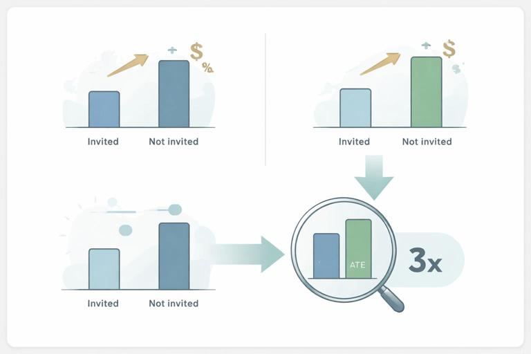
- The numerator is the “intention-to-treat” effect (ITT): the effect of being encouraged/assigned.
- The denominator is how much encouragement changes actual treatment uptake (the compliance rate difference).
If encouragement increases adoption by 10 percentage points and increases productivity by 0.5 units, then the implied effect of adoption among compliers is 0.5 / 0.10 = 5 units.
Important: if the denominator is tiny, the estimate explodes in variance and becomes fragile. This is why instrument strength matters.
Two-Stage Least Squares (2SLS): The Workhorse for Continuous Outcomes
For many business outcomes (revenue, time-on-task, number of tickets), a common approach is Two-Stage Least Squares (2SLS). Even if D is binary, 2SLS is widely used as an approximation and has a clear interpretation under standard IV assumptions.
Stage 1: Predict Treatment Using the Instrument
D = α + π Z + γ'X + uHere X are optional controls (e.g., baseline usage, region, device type). The fitted values D-hat represent the part of treatment explained by the instrument and controls.
Stage 2: Regress Outcome on Predicted Treatment
Y = β + τ D_hat + δ'X + ετ is the IV estimate of the causal effect of D on Y (for compliers, under monotonicity).
Practical note: you should not manually plug D-hat into an ordinary regression and use naive standard errors. Use an IV/2SLS procedure that computes correct standard errors (most stats packages do).
Step-by-Step: Designing an Encouragement IV Study
Step 1: Define the Treatment as “Received,” Not “Assigned”
Be explicit: D is the actual behavior (e.g., “used the dashboard at least once per week”), not the encouragement. Z is the lever (e.g., “received email + in-product banner”).
Step 2: Design the Instrument to Be Strong and Narrow
Strong: it should materially change uptake. Narrow: it should not affect the outcome through other channels.
- Use a message that is purely informational about how to access the feature, not motivational coaching.
- Avoid bundling multiple changes (e.g., don’t change pricing and send an email at the same time if pricing could directly affect outcomes).
- Consider multi-dose encouragement (e.g., email + banner) if a single nudge is too weak, but keep the content focused on access/awareness.
Step 3: Randomize the Instrument and Verify Balance
Randomly assign Z at the appropriate unit (user, account, team). Check that baseline covariates are similar across Z groups. While balance checks do not prove independence, large imbalances are a warning sign of implementation issues.
Step 4: Measure Compliance and Define the Compliance Window
Decide the time window in which D is considered “received” after Z. For example, adoption within 14 days of encouragement. Pre-registering this window internally helps avoid choosing a window that flatters results.
Step 5: Estimate ITT and First-Stage
Compute:
- ITT: difference in Y between Z=1 and Z=0.
- First-stage: difference in D between Z=1 and Z=0 (or regression coefficient π).
These two numbers already reveal whether the IV will be informative: if the first-stage is weak, you may need a stronger instrument or a different design.
Step 6: Compute IV/LATE and Robust Uncertainty
Use Wald (binary case) or 2SLS (general case). Use robust standard errors, and cluster if assignment or outcomes are correlated within groups (e.g., teams, accounts).
Step 7: Interpret as “Effect for Compliers” and Translate to Decisions
State clearly: “Among users whose adoption is changed by the encouragement, adopting the dashboard increases productivity by X.” Then connect it to a rollout lever: if your real-world policy is to send the encouragement broadly, LATE is directly relevant to the marginal users you will convert.
Imperfect Compliance in Classic Experiments: IV as a Fix for Noncompliance
Even when you run a randomized experiment, noncompliance can break the link between assignment and receipt. IV provides a principled way to estimate the effect of actually receiving the treatment, using assignment as the instrument.
Let Z be random assignment to treatment group, D be actual receipt (e.g., feature enabled and used), and Y be outcome. Then:
- ITT answers: “What is the effect of offering/enabling the treatment?”
- IV/LATE answers: “What is the effect of receiving/using the treatment for those induced to receive it by assignment?”
This is especially useful when treatment delivery fails (technical issues), when users can opt out, or when sales reps do not follow the assigned script.
Weak Instruments: The Most Common Failure Mode
A weak instrument means Z barely changes D. This creates two practical problems:
- High variance: confidence intervals become very wide, making the estimate unusable for decisions.
- Finite-sample bias: IV estimates can drift toward the biased non-IV estimate when instruments are weak, especially with many controls or small samples.
Practical mitigations:
- Strengthen the instrument (more salient encouragement, better delivery, multiple reminders) while guarding exclusion.
- Increase sample size (often necessary because IV is less statistically efficient than direct comparisons).
- Use limited controls that are clearly pre-treatment; avoid overfitting the first stage.
- Report first-stage strength transparently alongside the IV estimate.
Multiple Instruments and Overidentification (With Caution)
You can use multiple instruments (Z1, Z2, …) that each shift treatment. This can improve strength, but it also increases the burden of defending exclusion for each instrument.
With more instruments than endogenous treatments, you can run overidentification tests (e.g., Hansen’s J) that check whether instruments are mutually consistent. These tests can detect some violations, but they do not prove validity; instruments can fail in the same direction and still pass.
IV With Binary Outcomes and Nonlinear Models
Many business outcomes are binary (churn yes/no, conversion yes/no). Standard 2SLS is linear and can produce predictions outside [0,1], but it is often used as a reasonable approximation for average effects. Alternatives include:
- Two-stage residual inclusion (2SRI): often used with logistic models; requires careful assumptions and correct specification.
- Structural models / control function approaches: more complex, can be sensitive to modeling choices.
In practice, teams often start with linear IV for interpretability and robustness checks, then validate with alternative specifications if the decision is high-stakes.
Finding Instruments in Real Organizations: Patterns That Often Work
1) Randomized Encouragement
Most reliable because independence is built in. Examples: randomized reminders, in-product prompts, priority access, training invitations, default settings (if the default itself doesn’t directly affect outcomes beyond uptake).
2) Queueing and Capacity Constraints
Agent availability, server capacity, appointment slots, or random assignment to handlers can create quasi-random variation. You must control for time and routing rules to defend independence and exclusion.
3) Geographic or Timing Variation (Carefully)
Rollouts by region or time can be tempting instruments, but they often violate independence because regions and times differ in demand, competition, or seasonality. If used, you need strong controls and a credible argument that the rollout schedule is unrelated to outcome shocks.
4) Policy Rules That Affect Access but Not Outcomes Directly
Eligibility rules can sometimes act as instruments if they shift treatment uptake without directly changing outcomes, but many rules also change expectations or behavior directly. Be explicit about what the rule changes.
Practical Diagnostics and “Red Flag” Questions
Does Z change anything else besides D?
If the encouragement includes performance tips, it may directly affect Y. If agent availability changes wait time, and wait time affects churn independently of the call content, exclusion is threatened unless wait time is part of D.
Could Z be correlated with demand intensity or customer type?
Time-based instruments often correlate with demand. For example, “high availability” might occur during low-demand hours, and low-demand hours might have different churn patterns. You may need to include fine-grained time fixed effects or restrict to narrow windows.
Is the first-stage effect stable across segments?
If Z only moves D in a tiny niche, LATE pertains to that niche. That can still be valuable, but you should not generalize to the full population.
Is there evidence of defiers or reactance?
If some customers become less likely to adopt when nudged (e.g., they dislike marketing), monotonicity may fail. You can look for negative first-stage effects in subgroups as a warning.
Turning IV Results Into Business Actions
IV estimates are most actionable when the instrument resembles a scalable lever. If your instrument is “random email encouragement,” then the LATE is the effect for the marginal adopters you can create by sending that email. This can directly inform:
- Whether to invest in improving the onboarding flow (to increase compliance).
- Whether the product value is high enough among persuadable users to justify broader promotion.
- Forecasting impact: combine the estimated complier effect with expected adoption lift from scaled encouragement.
Be careful when the instrument is not a policy lever (e.g., agent availability). The estimate may still reveal the causal effect of the treatment, but translating it into a decision requires mapping how your real intervention would change treatment uptake and for whom.
Worked Numerical Example: Encouragement Email for Training Attendance
Scenario: You want the effect of attending a training session (D) on weekly sales (Y). Attendance is confounded by motivation. You randomize an invitation with a one-click calendar add (Z).
- Among Z=1 (invited), average sales Y is $12,200/week.
- Among Z=0 (not invited), average sales Y is $12,000/week.
- Attendance rate D among Z=1 is 30%.
- Attendance rate D among Z=0 is 20%.
Compute:
- ITT = 12,200 - 12,000 = $200/week.
- First-stage = 0.30 - 0.20 = 0.10.
- IV/LATE = 200 / 0.10 = $2,000/week increase in sales for compliers who attend because of the invitation.
Interpretation: the invitation increases sales a little on average because only 10% are induced to attend, but for those induced, the training effect is large. This suggests that improving compliance (e.g., better scheduling, manager support) could unlock more value.
Implementation Notes: Data, Logging, and Modeling Choices
Define D precisely and measure it reliably
IV is sensitive to mismeasurement of treatment receipt. If D is noisy (e.g., “used feature” measured inconsistently), the first-stage weakens and estimates degrade.
Use pre-treatment controls thoughtfully
Adding controls X can improve precision and adjust for chance imbalances, but controls should be clearly pre-treatment. Avoid post-instrument variables (e.g., engagement after encouragement) because they can introduce bias.
Cluster and stratify when appropriate
If Z is assigned at the team level, analyze at the team level or use clustered standard errors. If you stratified randomization (e.g., by region), include strata indicators in the model.
Report the full chain: Z→D and Z→Y
Decision-makers should see both the compliance lift and the ITT. The IV estimate alone can be misleading without context about how much the instrument actually moves behavior.