Why Randomize: What an RCT Adds Beyond “Good Data”
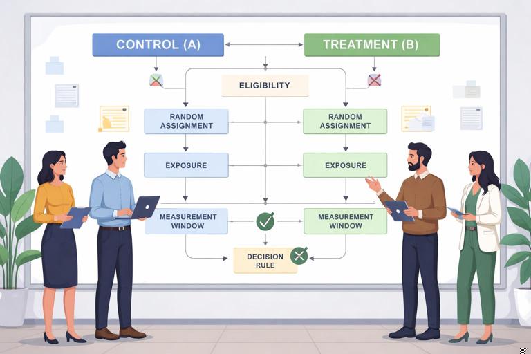
A randomized controlled trial (RCT) is an experiment where eligible units (users, customers, stores, sessions, leads, etc.) are assigned to different variants by chance, and outcomes are compared across variants. In business settings, the most common RCT format is an A/B test: A is the control (status quo) and B is a change (new design, offer, policy, algorithm, or message). Randomization is the mechanism that makes the groups comparable on average at the moment of assignment, so differences in outcomes can be attributed to the variant rather than to pre-existing differences.
In practice, the value of an RCT is not “it uses statistics,” but that it creates a clean comparison under controlled exposure. That control is operational: you decide who is eligible, when assignment happens, what each group experiences, what is measured, and how long the test runs. A well-designed RCT is therefore as much about product and operational discipline as it is about analysis.
Core Building Blocks of a Practical A/B Test
1) Unit of randomization (who gets assigned)
The unit is the entity that receives the treatment. Common units include user, account, device, session, household, store, call-center agent, or geographic region. Choose the unit that matches how the treatment is delivered and how outcomes are generated. If the treatment is a pricing policy applied at the account level, randomizing by session can cause the same account to see multiple prices, creating contamination and customer support issues.
- User-level: good for UI changes, messaging, onboarding flows; watch for cross-device identity issues.
- Session-level: fast, high volume; risk of the same user seeing both variants and learning effects.
- Cluster-level (store/region/team): needed when treatment is operational or when spillovers are likely; requires larger sample sizes and different analysis.
2) Eligibility and enrollment (who can be in the test)
Define inclusion and exclusion rules before launch. Eligibility should be based on information available prior to assignment. For example, “new visitors from paid search in the US on mobile” is acceptable if those attributes are known at assignment. Avoid rules that depend on post-assignment behavior (e.g., “users who clicked the banner”), because that can bias comparisons.
3) Treatment definition (what changes)
Specify exactly what differs between A and B: UI element, algorithm threshold, discount level, email subject line, shipping promise, or agent script. Keep the change as isolated as possible to reduce ambiguity in interpretation. If multiple changes must ship together, treat it as a bundled intervention and document the bundle.
- Listen to the audio with the screen off.
- Earn a certificate upon completion.
- Over 5000 courses for you to explore!

Download the app
4) Outcome measurement window (when you measure)
Decide the observation window: immediate (same session), short-term (7 days), or longer (28–90 days). The window should reflect the decision’s impact horizon. For subscription products, a 7-day window might capture activation but miss churn effects; for a checkout button color change, same-session conversion may be sufficient.
5) Estimand (what effect you want)
In business A/B testing, the most common estimand is the intention-to-treat (ITT) effect: compare outcomes by assigned group, regardless of whether users fully complied (e.g., saw the feature, opened the email). ITT matches many real decisions: “What happens if we roll this out with normal operational realities?” If you need the effect among compliers (those who actually received exposure), you must plan for it explicitly (e.g., with encouragement designs or instrumentation that supports compliance analysis) and accept additional assumptions.
Step-by-Step: Designing an A/B Test That Will Survive Reality
Step 1: Write a one-page experiment spec
Before building, write a short spec that includes: objective, variants, unit of randomization, eligibility, primary metric, guardrail metrics, assignment mechanism, ramp plan, duration, and decision rule. This document prevents “metric shopping” and mid-test redesigns that undermine interpretability.
Step 2: Choose a primary metric and guardrails
The primary metric is the single metric that determines success for the decision. Guardrails are metrics that must not degrade beyond a tolerance (e.g., refund rate, complaint rate, latency, unsubscribe rate, safety incidents). Keep the set small and pre-declared.
Practical guidance for metric choice:
- Prefer metrics close to the decision: If the change is in checkout, primary metric could be purchase conversion or revenue per visitor, not “time on site.”
- Use rate metrics carefully: Conversion rate is intuitive but can be noisy; revenue per user captures intensity but can be heavy-tailed.
- Define metric computation precisely: numerator/denominator, time window, handling of refunds, currency conversion, bot filtering, and deduplication rules.
Step 3: Decide the randomization and allocation strategy
Most tests use 50/50 allocation to maximize power for a fixed sample size. Unequal splits (e.g., 90/10) are used for risk management during ramp-up or when the treatment is expensive. If you plan a ramp (e.g., 1% → 10% → 50%), define the ramp criteria and ensure analysis accounts for time trends (often by analyzing only after reaching steady allocation, or by including time as a stratification variable).
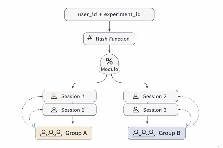
Implement random assignment using a stable hashing mechanism so that a unit stays in the same group across sessions (for user-level tests). For example, hash(user_id + experiment_id) mod 100 to assign buckets. Stability prevents cross-over and makes exposure consistent.
Step 4: Plan for interference, spillovers, and network effects
Many business environments violate the “no interference” ideal: one unit’s treatment can affect another’s outcome. Examples include social products (friends influence each other), marketplaces (sellers and buyers interact), and operations (a treated store changes inventory allocation affecting nearby stores).
Design options:
- Cluster randomization: assign by region/store/team to contain spillovers.
- Two-sided marketplace designs: randomize at the market level or use designs that treat both sides consistently.
- Holdout at higher level: keep some regions entirely control to capture equilibrium effects.
Interference is not just a statistical nuance; it changes what “rollout” means. If the product’s value depends on adoption, a small treatment fraction may understate full-rollout impact.
Step 5: Determine sample size, power, and minimum detectable effect (MDE)
Sample size planning forces clarity about what effect size is worth detecting. The MDE is the smallest effect you want a high probability of detecting (power), given a significance level (false positive tolerance). In practice, you choose MDE based on business value and feasibility: if you can only run for two weeks, you may not be able to detect a 0.1% lift in conversion reliably.
For a binary outcome (e.g., conversion), a common approximation for per-group sample size is:
n ≈ 2 * (z_(1-α/2) + z_(power))^2 * p(1-p) / (Δ)^2Where p is baseline conversion and Δ is the absolute lift you want to detect. For continuous outcomes (e.g., revenue per user), replace p(1-p) with the variance of the metric.
Practical tips:
- Use historical data to estimate baseline rates and variance.
- Account for heavy tails in revenue: consider winsorization, log transforms, or robust metrics (e.g., trimmed mean) if pre-specified.
- Adjust for clustering if randomizing by store/region: effective sample size is smaller due to intra-cluster correlation.
Step 6: Choose duration and handle seasonality
Duration should cover the full cycle relevant to the metric: at least one business cycle (often a full week) to capture weekday/weekend patterns, and longer if behavior changes slowly. If marketing campaigns, holidays, or product launches occur during the test, either avoid those periods or stratify and interpret carefully.
A common operational rule is: run until you reach planned sample size and you have covered at least one full weekly cycle, unless there is a safety stop.
Step 7: Instrumentation and logging (so you can trust the data)
Many A/B tests fail because the assignment and exposure are not logged correctly. At minimum, log:
- experiment_id, variant, assignment timestamp
- unit identifier (user_id/account_id) and eligibility flags
- exposure events (did the user actually see the feature?)
- outcome events with timestamps
Validate with a “dry run” or internal test: confirm that the split is correct, that users remain in the same bucket, and that metrics match known baselines.
Step 8: Predefine analysis rules (avoid peeking pitfalls)
Repeatedly checking results and stopping when p < 0.05 inflates false positives. If you need flexibility to stop early, use a sequential testing approach (e.g., alpha spending, group sequential designs) and define it before launch. If you do not have sequential methods in place, commit to a fixed horizon and avoid interpreting interim p-values as final.
Also predefine:
- how you handle missing data and late-arriving events
- how you treat outliers (if at all)
- which segments will be examined (exploratory vs decision-driving)
Common A/B Testing Designs in Business and When to Use Them
Parallel-group A/B (standard)
Users are assigned to A or B and remain there for the test. This is the default because it is simple and robust. It works well when carryover effects are minimal and when you can keep assignment stable.
Multi-armed tests (A/B/n)
More than one treatment variant is tested simultaneously (A vs B vs C). This can accelerate iteration but increases the risk of false positives due to multiple comparisons. Practical approaches include: controlling the family-wise error rate (e.g., Bonferroni/Holm) or using false discovery rate control when many variants are screened. Alternatively, use a staged approach: screen with smaller tests, then confirm with a focused A/B.
Factorial designs
Two or more factors are varied simultaneously (e.g., price display format × shipping message). Factorial designs can estimate main effects and interactions efficiently, but require careful planning and sufficient sample size to detect interactions, which are often smaller and noisier.
Switchback and time-based randomization
For operational systems where you cannot randomize individual units (e.g., delivery routing algorithm, call center queue policy), you can randomize by time blocks: alternate A and B by hour/day. This is useful when the system’s state is shared across units. The risk is time confounding (demand changes by time), so you typically randomize many blocks and balance across days of week.
Cluster randomized trials
Randomize groups (stores, regions, classrooms, sales teams). Use when spillovers are likely or when treatment is delivered at the group level. Plan for reduced power and analyze with cluster-robust methods. Also ensure enough clusters; having many users but only a few clusters can still yield unreliable inference.
Operational Threats to Valid A/B Tests (and How to Prevent Them)
Sample ratio mismatch (SRM)
SRM occurs when the observed allocation deviates from the intended split (e.g., 50/50 planned but 55/45 observed). This often indicates a bug: eligibility differs by variant, assignment is not stable, or logging is broken. SRM is a launch-blocker: investigate before trusting outcome differences.
Noncompliance and partial exposure
Users may be assigned to B but never see it due to caching, feature flags, app version, or ad blockers. ITT remains valid for the rollout decision, but the effect may look diluted. Track exposure rates and diagnose why users are not receiving the intended experience.
Novelty and learning effects
Some changes create a short-term spike (novelty) or dip (learning curve) that fades. If you decide too early, you may ship a change that harms steady-state performance or reject one that would have improved after adaptation. Mitigate by choosing an appropriate duration and by examining metric trajectories over time (pre-specified as diagnostic, not as a reason to stop early without a plan).
Carryover effects
If users can be exposed to both variants over time (e.g., session-level assignment), earlier exposure can influence later outcomes. Prefer stable user-level assignment when behavior can persist (preferences, habit formation, saved carts).
Instrumentation changes mid-test
Changing event definitions, deduplication logic, or attribution windows during a test can create artificial differences. Freeze metric definitions for the test period, or version your metrics so analysis uses consistent logic.
Interpreting Results for Decisions: Effect Sizes, Uncertainty, and Tradeoffs
Report absolute and relative effects
For conversion, report both absolute lift (e.g., +0.4 percentage points) and relative lift (e.g., +5%). Absolute effects connect to volume and revenue; relative effects help compare across baselines.
Use confidence intervals, not just p-values
A p-value answers a narrow question about compatibility with a null effect under assumptions. Decision-making benefits from an interval: “Given the data, plausible effects range from X to Y.” If the interval includes meaningful harm, you may not ship even if the point estimate is positive.
Guardrail tradeoffs
Sometimes the primary metric improves while a guardrail degrades. Predefine acceptable thresholds (e.g., “refund rate must not increase by more than 0.2 percentage points”). If thresholds are not predeclared, teams can rationalize outcomes after the fact.
Segment analysis: exploratory vs confirmatory
It is tempting to search for “the segment where it works.” Treat post-hoc segment findings as hypotheses for a follow-up test. If you must make a segmented decision (e.g., roll out only to new users), plan that segmentation in advance and power the test accordingly.
Worked Practical Example: Checkout Change A/B Test
Scenario: You want to add an express checkout button on the cart page.
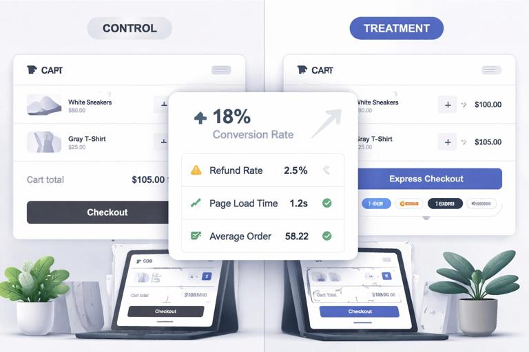
- Unit: user_id (stable across sessions)
- Eligibility: logged-in users in US/CA on web who reach cart page
- Variants: A = current cart; B = cart with express checkout button
- Primary metric: purchase conversion within 24 hours of first cart view
- Guardrails: refund rate within 14 days, payment failures, page load time
- Allocation: ramp 1% for 6 hours (monitor errors) → 10% for 24 hours → 50/50
- Duration: until sample size reached and at least 14 days to capture refunds
- Analysis plan: ITT comparison of conversion; cluster-robust not needed (user-level); sequential testing not used, so no early stopping for wins
Implementation checks: verify SRM daily; verify exposure event fires when cart renders; verify that users remain in same bucket; verify that express checkout is actually available (e.g., payment method eligibility) and log reasons when unavailable.
Decision framing: If conversion improves and guardrails stay within thresholds, ship. If conversion improves but refunds increase beyond threshold, consider shipping with additional friction checks or limiting to low-risk payment methods, then retest.
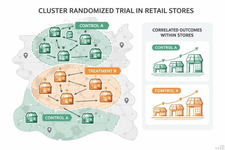
Worked Practical Example: Store-Level Operational Change (Cluster RCT)
Scenario: A retailer wants to test a new shelf-restocking schedule intended to reduce stockouts.
- Unit: store (cluster randomization)
- Eligibility: stores with similar size and baseline stockout rates; exclude stores under renovation
- Variants: A = current schedule; B = new schedule
- Primary metric: stockout minutes per day (or % of SKUs stocked out)
- Guardrails: labor hours, overtime, employee turnover, customer complaints
- Allocation: 50/50 across stores, stratified by region and store size to balance key drivers
- Duration: 8 weeks to cover replenishment cycles and promotions
Key design adjustment: Because outcomes within a store are correlated, you need enough stores, not just enough transactions. Plan sample size using an estimate of intra-store correlation and analyze with cluster-robust standard errors or mixed models.
Practical Checklists
Pre-launch checklist
- Experiment spec written and approved (primary metric + guardrails predeclared)
- Randomization unit matches treatment delivery; stable assignment implemented
- Eligibility defined using pre-assignment information
- Instrumentation validated: assignment, exposure, outcomes, timestamps
- SRM monitoring in place
- Ramp plan and safety stop criteria defined
- Sample size/MDE and duration planned (including weekly cycle)
In-test checklist
- Monitor SRM, errors, latency, and exposure rates
- Avoid mid-test changes to variants or metric definitions
- Do not stop early without a pre-specified sequential plan or safety reason
- Track external events (campaigns, outages) that may affect interpretation
Post-test checklist
- Compute ITT effect with confidence intervals
- Check guardrails against thresholds
- Validate data integrity (no logging gaps, stable assignment, consistent eligibility)
- Treat unplanned segment findings as hypotheses for follow-up tests