Heterogeneous Effects and Personalization with Uplift Modeling

Why average treatment effect is not enough

Many business decisions are not about whether a treatment works “on average,” but about who it works for and where it might backfire. A discount might increase purchases for price-sensitive customers while reducing margin for loyal customers who would have bought anyway. A new onboarding flow might help novices but confuse experienced users. When effects vary across people, contexts, or time, the overall average can hide the most important operational insight: which segments should receive the intervention and which should not.

This chapter focuses on heterogeneous treatment effects (HTE) and uplift modeling (also called incremental response modeling). The goal is personalization: assign treatments to individuals (or accounts, stores, regions) to maximize expected business value while controlling risk and constraints.

Heterogeneous treatment effects: what varies and why it matters

Heterogeneous effects mean the causal effect of a treatment differs across units. Instead of a single number, we care about a function: the conditional average treatment effect (CATE), often written as τ(x), the expected treatment effect for units with features x.

Examples of heterogeneity that commonly matters in business:

• Customer lifecycle: new vs. returning users may respond differently to onboarding, messaging, or pricing.
• Baseline propensity: users already likely to convert may show little incremental lift; low-propensity users might show higher lift (or none).
• Channel and context: email vs. push vs. in-app; mobile vs. desktop; weekday vs. weekend.
• Capacity constraints: a support intervention may help most when support load is low; when load is high, it could worsen outcomes.
• Risk and harm: a credit offer might increase revenue for some but increase default risk for others.

Personalization is the decision layer on top of heterogeneity: if you can estimate τ(x), you can choose to treat when τ(x) is positive (or exceeds a threshold that accounts for cost and risk).

Continue in our app.

• Listen to the audio with the screen off.
• Earn a certificate upon completion.
• Over 5000 courses for you to explore!

Or continue reading below...

Download the app

What uplift modeling is (and what it is not)

Uplift modeling directly targets the incremental effect of a treatment on an outcome for each unit. It differs from standard predictive modeling in a crucial way:

• Predictive model: estimates P(Y=1 | X=x) or E[Y | X=x]. It tells you who is likely to convert, not who will convert because of the treatment.
• Uplift model: estimates the difference between treated and untreated outcomes conditional on X: τ(x) = E[Y | T=1, X=x] − E[Y | T=0, X=x]. It tells you who is likely to change because of the treatment.

This distinction prevents a common mistake: targeting “high likelihood to buy” customers with promotions. Those customers may buy anyway, creating low incremental lift and unnecessary cost. Uplift modeling aims to find persuadables (positive uplift), avoid sure things (low uplift), and avoid do-not-disturb groups (negative uplift).

The four intuitive response types

For binary outcomes like conversion, uplift thinking often uses four conceptual types:

• Persuadables: convert only if treated (positive uplift).
• Sure things: convert regardless (near-zero uplift).
• Lost causes: do not convert regardless (near-zero uplift).
• Sleeping dogs: convert only if not treated (negative uplift; treatment harms).

You cannot observe these types for an individual directly, but uplift models try to infer them probabilistically from randomized data and features.

From uplift to decisions: value, costs, and constraints

In practice, you rarely treat based on uplift alone. You treat based on expected net value. A simple decision rule is:

Treat if V(x) = τ(x) × Benefit − Cost − RiskPenalty > 0

Where:

• Benefit could be incremental gross profit per conversion, incremental retention value, or incremental revenue adjusted for margin.
• Cost could be discount amount, incentive cost, operational cost, or opportunity cost.
• RiskPenalty could represent expected increase in churn, complaints, fraud, or regulatory risk.

Constraints also matter: limited budget, limited inventory, limited contact frequency, fairness constraints, or capacity constraints. This turns personalization into an optimization problem: treat the subset of users with the highest expected net value subject to constraints.

Practical step-by-step workflow for uplift personalization

Step 1: Define the decision and the treatment options

Be explicit about what you can choose. Examples:

• Send a retention email vs. do nothing.
• Offer 10% discount vs. 0% discount.
• Show onboarding checklist vs. standard onboarding.

If there are multiple treatments (e.g., 5%, 10%, free shipping), uplift becomes multi-treatment. Start with a binary treatment if possible to build intuition and reduce complexity.

Step 2: Choose outcomes and value metrics aligned to the decision

Pick an outcome that reflects the business objective and is measurable within a reasonable time window. Common choices:

• Conversion within 7 days
• Incremental revenue within 14 days
• Retention at day 30

Also define a value mapping: how does a unit change in the outcome translate to profit or utility? For example, if the outcome is conversion, estimate margin per conversion; if the outcome is revenue, use contribution margin; if the outcome is retention, use expected lifetime value uplift.

Step 3: Collect data that supports individualized effect estimation

Uplift modeling is most reliable when trained on randomized experiments (or well-designed quasi-experiments) where treatment assignment is independent of potential outcomes given features. In a randomized setting, you can estimate uplift without needing to model selection into treatment.

Data requirements:

• Treatment indicator: who was treated.
• Outcome: observed result.
• Features X: pre-treatment covariates only (no leakage from post-treatment behavior).
• Exposure/logging integrity: ensure the treatment was actually delivered and recorded.

Feature examples for personalization: tenure, past purchases, browsing frequency, device, region, prior engagement, subscription status, price sensitivity proxies, and customer support history (if pre-treatment).

Step 4: Split data for honest evaluation

Because uplift models can overfit subtle differences between treated and control groups, evaluation must be done on held-out data. Use:

• Train/validation/test split, or cross-fitting.
• Stratification by treatment assignment to preserve balance.
• Time-based splits when behavior drifts over time.

Step 5: Choose an uplift modeling approach

There are several families of methods. The right choice depends on data size, feature complexity, and interpretability needs.

Approach A: Two-model (T-learner) uplift

Train two separate predictive models:

• Model 1 estimates E[Y | T=1, X]
• Model 0 estimates E[Y | T=0, X]

Then uplift is the difference of predictions. This is simple and flexible but can be noisy when one group is small or when models extrapolate differently.

# Pseudocode for T-learner uplift scoring
fit model_t on data where T=1: predict y from X
fit model_c on data where T=0: predict y from X
for each user i:
  mu1 = model_t.predict(X_i)
  mu0 = model_c.predict(X_i)
  uplift_i = mu1 - mu0

Approach B: Single-model with treatment interaction (S-learner)

Train one model that takes X and T as inputs and includes interactions (implicitly via tree-based models or explicitly via feature crosses). Then compute uplift by predicting twice: once with T=1 and once with T=0.

This can be stable when data is limited, but it may understate heterogeneity if the model learns that T has a mostly constant effect.

# Pseudocode for S-learner
fit model on all data: predict y from [X, T]
for each user i:
  mu1 = model.predict([X_i, T=1])
  mu0 = model.predict([X_i, T=0])
  uplift_i = mu1 - mu0

Approach C: Transformed outcome / uplift trees

Some methods transform the outcome so that a single supervised model can target uplift directly (common in uplift trees and certain meta-learners). Tree-based uplift models can produce interpretable segments with different estimated uplift, which is useful for stakeholder communication and policy constraints.

Interpretability advantage: you can explain uplift using a small number of splits (e.g., “new users with low prior engagement show +3pp uplift; high-engagement users show −1pp uplift”).

Approach D: Meta-learners for CATE (X-learner, R-learner, DR-learner)

These approaches are designed to estimate CATE more efficiently, especially when treatment and control sizes differ or when outcomes are noisy. They often combine outcome modeling and propensity information (even in randomized settings, propensity is known). In practice, these methods can outperform simple two-model approaches when data is moderate and heterogeneity is subtle.

Implementation detail: many teams use libraries that provide these learners; the key operational point is to keep the training and evaluation protocol honest and to validate uplift with uplift-specific metrics.

Step 6: Evaluate uplift models with uplift-aware metrics

Standard metrics like AUC for conversion prediction do not measure incremental impact. You need metrics that reflect how well the model ranks users by true uplift.

Uplift/Qini curve intuition

Sort users by predicted uplift from highest to lowest. Consider treating the top k% and compute the incremental outcome (treated minus control) within that prefix. Plot incremental gain vs. fraction targeted. A good uplift model produces a curve that rises steeply early (high uplift concentrated at the top).

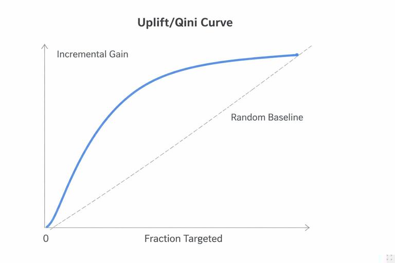
Common summary metrics:

• Qini coefficient: area between the model’s Qini curve and a baseline (random targeting).
• AUUC (Area Under the Uplift Curve): integrates uplift over targeting fractions.

Practical evaluation checklist:

• Compute uplift curves on a held-out test set.
• Use confidence intervals via bootstrap because uplift estimates can be noisy.
• Check stability across time, channels, and key subgroups.

Calibration for decision-making

Ranking is often enough for targeting a fixed budget (treat top N). But if you need a threshold rule (treat if uplift > 0), you need calibrated uplift estimates. Calibration is harder for uplift than for probabilities. A practical approach is to:

• Bin users by predicted uplift deciles.
• Within each bin, estimate observed incremental effect using treated vs. control.
• Use these bin-level estimates as a calibrated lookup table for policy decisions.

Step 7: Turn uplift scores into a treatment policy

Common policies:

• Top-k targeting: treat the top k% by predicted net value.
• Threshold targeting: treat if predicted net value > 0.
• Budgeted optimization: maximize total expected value subject to cost constraints (e.g., total discount spend).
• Risk-constrained targeting: treat only if uplift is positive and predicted risk uplift (e.g., churn) is below a threshold.

When costs vary by user (e.g., discount proportional to basket size), compute expected net value per user and rank by that, not by uplift alone.

Step 8: Validate the personalization policy with a policy test

After training an uplift model, you still need to validate that the policy improves outcomes when deployed. A practical design is a two-level experiment:

• Holdout group: business-as-usual targeting (or random targeting).
• Personalization group: apply the uplift-based policy.

Within the personalization group, you may still randomize treatment for a small fraction to keep learning (exploration) and to detect drift. This is especially important when user behavior changes or when the treatment effect depends on external factors.

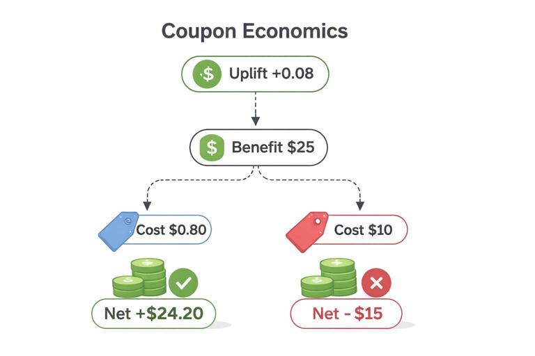
Practical example: discount targeting without wasting margin

Scenario: You can offer a $10 coupon to encourage purchase within 7 days. The coupon costs $10 in margin when redeemed. The average order margin is $25. You want to send coupons only when incremental purchases justify the cost.

Define:

• Outcome Y: purchase within 7 days (0/1)
• Benefit per incremental purchase: $25 margin
• Cost per treated user: expected coupon cost = $10 × P(redeem | treated, X) (or approximate as $10 if redemption is near-certain upon purchase)

Suppose your uplift model predicts τ(x)=+0.08 for a segment (8 percentage point increase in purchase probability). Expected incremental margin = 0.08 × $25 = $2.00. If expected coupon cost is $0.80 (because only 8% incremental purchases redeem, and baseline redeems are handled carefully), net value might be positive. But if coupon cost is closer to $10 for everyone treated, net value is negative. This illustrates why you should model value carefully: uplift in conversion is not automatically profit uplift.

Operationally, many teams model two uplifts: uplift on purchase and uplift on discount redemption (or average discount cost), then compute expected profit uplift.

Common pitfalls and how to avoid them

Targeting high propensity instead of high uplift

A model that predicts conversion probability will often rank “sure things” at the top. If you target them, you pay incentive costs with little incremental gain. Always evaluate with uplift curves, not just conversion lift in the treated group.

Feature leakage from post-treatment behavior

If you include features that are affected by treatment (e.g., “number of sessions after email send”), the model will learn patterns that cannot be used at decision time and will inflate offline performance. Use only pre-treatment features available at the moment you decide.

Small effective sample sizes

Uplift is a difference between two conditional expectations, so it is noisier than prediction. If you slice too finely, estimates become unstable. Practical mitigations:

• Start with fewer, stronger features.
• Use regularized models or tree constraints.
• Prefer methods designed for CATE stability (e.g., DR-style learners) when appropriate.
• Report uncertainty at segment level (e.g., deciles) rather than per-user point estimates.

Negative uplift segments and harm

Negative uplift is not just “no effect”; it can represent harm (e.g., increased churn due to too many messages). Treat negative uplift as a first-class outcome: build guardrails into the policy (do not treat if predicted uplift is negative; cap frequency; add risk models).

Changing effects over time (drift)

Personalization policies can change user composition and behavior. Also, seasonality and competitive dynamics can shift effects. Mitigations:

• Monitor uplift curves over time on fresh randomized data.
• Retrain on a cadence aligned with drift (weekly/monthly/quarterly).
• Keep a small randomized exploration bucket to continuously measure incremental effects.

Multi-treatment uplift and choosing among options

Many real decisions involve more than “treat vs. not treat”: different creatives, channels, or incentive levels. Multi-treatment uplift aims to estimate which option yields the highest expected value for each user.

Practical approach:

• Run an experiment with multiple arms (including control).
• Estimate CATE for each treatment vs. control: τ_k(x) for treatment k.
• Compute expected net value for each option: V_k(x).
• Choose argmax over k, including the option “do nothing.”

Be careful with multiple comparisons and data fragmentation: each additional arm reduces sample per arm. If data is limited, consider a staged approach: first identify whether incentives help at all, then personalize incentive levels among responders.

Operationalizing uplift: from model to production policy

Scoring and decision service

At decision time (e.g., when a user visits the app), you need:

• Feature computation that matches training (same definitions, same time windows).
• Model scoring to produce uplift or net value.
• A policy layer that applies constraints (budget, frequency caps, eligibility rules).

Keep the policy logic separate from the model so business rules can evolve without retraining.

Monitoring: what to track

Monitoring should cover both model health and causal performance:

• Data drift: feature distributions, missingness, eligibility rates.
• Score drift: distribution of predicted uplift/net value.
• Policy outputs: fraction treated, spend, channel mix.
• Incremental impact: measured via ongoing randomized holdout or periodic policy tests.

Documentation for stakeholders

Uplift models can be harder to trust than standard predictors. Provide artifacts that connect model outputs to business outcomes:

• Uplift/Qini curves with confidence intervals.
• Decile tables showing observed incremental outcomes and net value.
• Top segments with positive and negative uplift and their defining characteristics.
• Clear eligibility and exclusion rules to prevent unintended targeting.

Hands-on checklist you can apply to your next personalization project

• Write the decision rule in terms of expected net value, not just uplift.
• Use only pre-treatment features available at decision time.
• Train at least one baseline uplift method (T-learner or S-learner) before more complex learners.
• Evaluate with uplift-aware curves (Qini/AUUC) on a held-out set.
• Calibrate uplift at the segment/decile level if you need thresholds.
• Deploy as a policy with constraints (budget, frequency, risk guardrails).
• Validate with a policy test and keep a small exploration bucket for continuous measurement.