Hands-On Python Workflows with pandas and statsmodels

What This Chapter Delivers: Reproducible Causal Workflows in Python

This chapter focuses on the mechanics of building reliable, repeatable analysis pipelines in Python using pandas for data preparation and statsmodels for estimation and inference. The goal is not to re-explain causal concepts, but to show how to implement common estimation patterns, diagnostics, and reporting in a way that is auditable and production-friendly. You will learn how to: (1) structure data for analysis, (2) create clean design matrices, (3) fit models with robust standard errors, (4) compute interpretable effect summaries, and (5) package the workflow so it can be rerun on new data without manual steps.

Environment Setup and Project Structure

For consistent results, pin versions and keep analysis code separate from data. A minimal setup uses a virtual environment and a small project layout.

Recommended folder layout

• data/ (raw extracts, read-only)
• notebooks/ (exploration, optional)
• src/ (reusable functions: cleaning, modeling, reporting)
• reports/ (tables, figures, model summaries)

Core imports

import numpy as np
import pandas as pd
import statsmodels.api as sm
import statsmodels.formula.api as smf

from patsy import dmatrices

In practice, you will also want pyarrow for fast parquet IO and matplotlib/seaborn for plots, but the core workflow here stays within pandas and statsmodels.

Data Ingestion and “Analysis-Ready” Tables

Most modeling issues come from messy inputs: duplicated rows, inconsistent types, missingness, and incorrect unit of analysis. A reliable workflow starts by creating an “analysis-ready” table with one row per unit (user, order, store-day, etc.), with clearly typed columns.

Step-by-step: load, validate, and type-cast

df = pd.read_parquet("data/events.parquet")

# Basic checks
assert df.shape[0] > 0
assert df["user_id"].notna().all()

# Type casting
df["event_time"] = pd.to_datetime(df["event_time"], utc=True)
df["treatment"] = df["treatment"].astype(int)

# Example: ensure numeric outcome
df["revenue"] = pd.to_numeric(df["revenue"], errors="coerce")

Prefer explicit casting over relying on inferred dtypes. If a column is supposed to be binary, force it to int and validate it contains only 0/1.

Continue in our app.

• Listen to the audio with the screen off.
• Earn a certificate upon completion.
• Over 5000 courses for you to explore!

Or continue reading below...

Download the app

Unit-of-analysis aggregation with pandas

Suppose you have event-level data but want user-level outcomes over a window. Aggregate carefully and keep the aggregation logic in code (not in ad hoc spreadsheet steps).

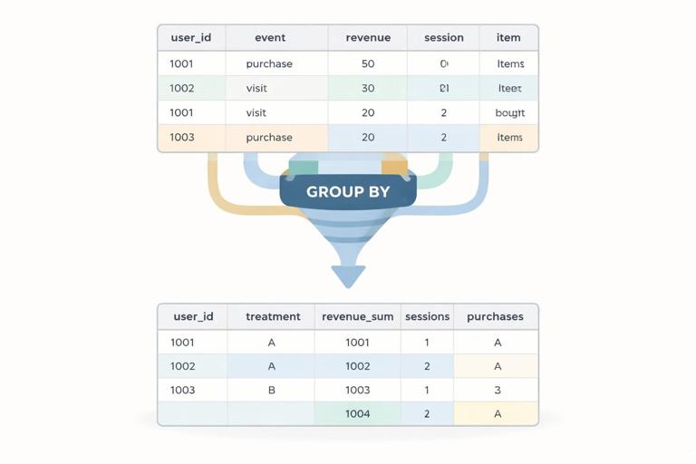
# Example: user-level table over a post period
user_df = (df
    .groupby(["user_id", "treatment"], as_index=False)
    .agg(
        revenue_sum=("revenue", "sum"),
        sessions=("session_id", "nunique"),
        purchases=("purchase_id", "nunique"),
        first_event=("event_time", "min"),
        last_event=("event_time", "max"),
    )
)

Common pitfalls to guard against: (1) mixing pre and post windows, (2) double-counting due to joins, and (3) inadvertently conditioning on post-treatment variables during feature creation. Keep feature engineering aligned with your intended design and document each derived column.

Handling Missing Data and Outliers with Transparent Rules

Statsmodels will typically drop rows with missing values in any variable used in the model. That can silently change your sample. Make missingness handling explicit and report how many rows are removed.

Step-by-step: explicit missingness policy

model_cols = ["revenue_sum", "treatment", "sessions"]

before = user_df.shape[0]
model_df = user_df.dropna(subset=model_cols).copy()
after = model_df.shape[0]

dropped = before - after

For outliers, avoid arbitrary trimming without justification. If you do winsorize, implement it deterministically and store both raw and capped versions.

def winsorize_series(s, p=0.99):
    cap = s.quantile(p)
    return s.clip(upper=cap)

model_df["revenue_w"] = winsorize_series(model_df["revenue_sum"], p=0.99)

Design Matrices: From pandas Columns to Model Inputs

Statsmodels supports two main interfaces: (1) the “array” interface where you manually build X and y, and (2) the formula interface using Patsy (recommended for readability and categorical handling). Use formulas when you want clear, auditable model specifications.

Formula interface basics

# Simple linear model: outcome ~ treatment + covariates
res = smf.ols("revenue_w ~ treatment + sessions", data=model_df).fit()
print(res.summary())

For categorical variables, use C(var). Patsy will create dummy variables with a reference category.

res = smf.ols("revenue_w ~ treatment + sessions + C(country)", data=model_df).fit()

Array interface (useful for custom pipelines)

y = model_df["revenue_w"].to_numpy()
X = model_df[["treatment", "sessions"]].to_numpy()
X = sm.add_constant(X)

res = sm.OLS(y, X).fit()

The array interface is more verbose but can be easier to integrate into reusable functions when you already have a prepared numeric matrix.

Robust Standard Errors and Clustered Inference

Business data often violates the ideal assumptions of homoskedastic, independent errors. Statsmodels makes it straightforward to request robust covariance estimators. This is a workflow habit: fit the model, then choose an appropriate covariance type for inference.

Heteroskedasticity-robust (HC) standard errors

res = smf.ols("revenue_w ~ treatment + sessions", data=model_df).fit(cov_type="HC3")

HC3 is a common default in applied work, especially with moderate sample sizes.

Cluster-robust standard errors

If outcomes are correlated within clusters (e.g., users within stores, repeated measures within users, or geo-level rollouts), cluster-robust inference is often more appropriate.

res = smf.ols("revenue_w ~ treatment + sessions", data=model_df).fit(
    cov_type="cluster",
    cov_kwds={"groups": model_df["store_id"]}
)

Make sure the clustering variable is aligned with how correlation arises. If you cluster at store level, you need enough stores for stable inference; otherwise, consider alternative designs or aggregation.

Interpreting Model Outputs as Decision-Ready Effect Summaries

Model summaries can be overwhelming for stakeholders. A practical workflow extracts the treatment coefficient, standard error, confidence interval, and a few derived metrics (like percent lift relative to baseline).

Step-by-step: extract treatment effect and CI

coef = res.params["treatment"]
se = res.bse["treatment"]
ci_low, ci_high = res.conf_int().loc["treatment"].tolist()

summary = {
    "ate": float(coef),
    "se": float(se),
    "ci_low": float(ci_low),
    "ci_high": float(ci_high),
    "p_value": float(res.pvalues["treatment"]),
}

Percent lift relative to control mean

control_mean = model_df.loc[model_df["treatment"] == 0, "revenue_w"].mean()
summary["control_mean"] = float(control_mean)
summary["pct_lift"] = float(coef / control_mean) if control_mean != 0 else np.nan

Percent lift is often easier to communicate than raw dollars, but always report the baseline used and ensure it is computed on the same analysis sample.

Binary Outcomes: Logistic Regression with statsmodels

When the outcome is binary (e.g., converted vs not), use logistic regression. Statsmodels provides logit via the formula API. Coefficients are in log-odds, so you typically convert to odds ratios or compute marginal effects.

Fit a logistic regression

model_df["converted"] = (model_df["purchases"] > 0).astype(int)

logit_res = smf.logit("converted ~ treatment + sessions + C(country)", data=model_df).fit(disp=False)

Odds ratio for treatment

or_treat = float(np.exp(logit_res.params["treatment"]))

Average marginal effect (more interpretable)

mfx = logit_res.get_margeff(at="overall")
# Convert to a tidy table
mfx_df = mfx.summary_frame()

The marginal effect for treatment approximates the average change in conversion probability when switching from control to treatment, holding other variables at their observed values (depending on the marginal effects settings).

Count Outcomes: Poisson and Negative Binomial Models

For count outcomes (e.g., number of purchases, number of tickets), linear regression can be a poor fit. Statsmodels supports generalized linear models (GLMs) such as Poisson and Negative Binomial.

Poisson GLM

pois_res = smf.glm(
    "purchases ~ treatment + sessions + C(country)",
    data=model_df,
    family=sm.families.Poisson()
).fit(cov_type="HC3")

Poisson coefficients are on the log scale; exponentiating gives multiplicative effects on the expected count.

mult = float(np.exp(pois_res.params["treatment"]))

Negative Binomial for overdispersion

nb_res = smf.glm(
    "purchases ~ treatment + sessions + C(country)",
    data=model_df,
    family=sm.families.NegativeBinomial(alpha=1.0)
).fit(cov_type="HC3")

In practice, you may compare Poisson vs Negative Binomial fit using residual diagnostics and whether variance greatly exceeds the mean.

Fixed Effects Patterns with Categorical Controls

Many business datasets have systematic differences by time (day/week), geography, product category, or seller. A practical implementation pattern is to include fixed effects via categorical variables in the formula. This is straightforward but can create many dummy columns, so monitor memory and runtime.

Example: time and geo fixed effects

fe_res = smf.ols(
    "revenue_w ~ treatment + sessions + C(week) + C(region)",
    data=model_df
).fit(cov_type="HC3")

If you have a very high-cardinality fixed effect (e.g., user_id), statsmodels OLS with dummies may be too heavy. In those cases, consider aggregating to a higher level, using within-transformation workflows, or specialized estimators; but for many business settings, week and region fixed effects are manageable.

Reusable Modeling Functions: One Pipeline, Many Metrics

A common need is to run the same specification across multiple outcomes (revenue, retention, support contacts) and produce a consistent table. Write a small function that takes a dataframe, formula, and covariance settings, then returns a tidy row.

Step-by-step: build a tidy result row

def fit_ols_tidy(data, formula, treat_var="treatment", cov_type="HC3", cluster=None):
    if cov_type == "cluster":
        res = smf.ols(formula, data=data).fit(
            cov_type="cluster",
            cov_kwds={"groups": data[cluster]}
        )
    else:
        res = smf.ols(formula, data=data).fit(cov_type=cov_type)

    coef = res.params[treat_var]
    ci = res.conf_int().loc[treat_var].tolist()

    return {
        "formula": formula,
        "n": int(res.nobs),
        "ate": float(coef),
        "ci_low": float(ci[0]),
        "ci_high": float(ci[1]),
        "p_value": float(res.pvalues[treat_var]),
        "cov_type": cov_type,
    }

rows = []
rows.append(fit_ols_tidy(model_df, "revenue_w ~ treatment + sessions + C(country)", cov_type="HC3"))
rows.append(fit_ols_tidy(model_df, "sessions ~ treatment + C(country)", cov_type="HC3"))

results_df = pd.DataFrame(rows)

This pattern makes it easy to export results to CSV and keep a record of exactly what was run.

Diagnostics You Can Automate

Even when you are focused on effect estimation, basic diagnostics help catch data and modeling issues early. Automate checks so they run every time.

Residual checks (quick sanity)

model_df["resid"] = res.resid

# Large residuals might indicate data issues
bad = model_df.loc[model_df["resid"].abs() > model_df["resid"].abs().quantile(0.999)]

Influence and leverage

infl = res.get_influence()
summary_infl = infl.summary_frame()

# Cook's distance as a quick flag
model_df["cooks_d"] = summary_infl["cooks_d"].to_numpy()

Influence diagnostics are not a reason to automatically delete points, but they help you identify whether a small number of observations dominate the estimate due to extreme outcomes or data errors.

Reporting: Exporting Tables That Stakeholders Can Read

Statsmodels summaries are useful for analysts, but decision workflows benefit from compact tables: effect, CI, p-value, baseline, and sample size. Use pandas to format and export.

Step-by-step: create a stakeholder table

def format_effect_table(data, outcome, formula):
    res = smf.ols(formula, data=data).fit(cov_type="HC3")
    coef = res.params["treatment"]
    ci_low, ci_high = res.conf_int().loc["treatment"].tolist()
    control_mean = data.loc[data["treatment"] == 0, outcome].mean()

    return pd.DataFrame([{
        "outcome": outcome,
        "n": int(res.nobs),
        "control_mean": float(control_mean),
        "effect": float(coef),
        "ci_low": float(ci_low),
        "ci_high": float(ci_high),
        "pct_lift": float(coef / control_mean) if control_mean != 0 else np.nan,
        "p_value": float(res.pvalues["treatment"]),
    }])

table = format_effect_table(model_df, "revenue_w", "revenue_w ~ treatment + sessions + C(country)")
table.to_csv("reports/effects.csv", index=False)

Keep the exact formula string in the exported output or in metadata so results are traceable. In regulated or high-stakes environments, traceability is as important as the estimate.

Workflow Pattern: One Notebook for Exploration, One Script for Production

A practical approach is to explore in a notebook, then move stable steps into scripts or functions. The notebook helps you iterate quickly; the script ensures reproducibility.

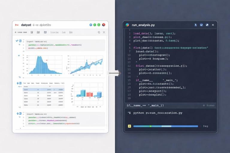
Example: a minimal “run_analysis.py” flow

def load_data(path):
    df = pd.read_parquet(path)
    df["event_time"] = pd.to_datetime(df["event_time"], utc=True)
    df["treatment"] = df["treatment"].astype(int)
    df["revenue"] = pd.to_numeric(df["revenue"], errors="coerce")
    return df

def make_user_table(df):
    user_df = (df
        .groupby(["user_id", "treatment"], as_index=False)
        .agg(revenue_sum=("revenue", "sum"), sessions=("session_id", "nunique"))
    )
    user_df["revenue_w"] = winsorize_series(user_df["revenue_sum"], p=0.99)
    return user_df

def run_models(user_df):
    user_df = user_df.dropna(subset=["revenue_w", "treatment", "sessions"]).copy()
    res = smf.ols("revenue_w ~ treatment + sessions", data=user_df).fit(cov_type="HC3")
    return res

# Orchestrate
raw = load_data("data/events.parquet")
user_df = make_user_table(raw)
res = run_models(user_df)

This pattern makes it easy to rerun the same analysis on a new date range or a new market by changing only the input path or a configuration variable.

Common Implementation Mistakes (and How to Prevent Them)

1) Silent row dropping due to missing values

Prevention: always compute before/after row counts when you create model_df, and log the number dropped per column.

2) Wrong join keys creating duplication

Prevention: after merges, check row counts and uniqueness constraints.

merged = user_df.merge(dim_df, on="user_id", how="left")
assert merged.shape[0] == user_df.shape[0]

3) Treating strings as categories inconsistently

Prevention: standardize casing and missing labels.

model_df["country"] = model_df["country"].fillna("UNKNOWN").str.upper()

4) Interpreting coefficients without checking scale

Prevention: store units in column names (e.g., revenue_usd, minutes_spent) and compute baseline means alongside effects.

Putting It Together: A Repeatable “Effect Estimation” Template

When you need to run multiple analyses quickly, a template reduces errors. The template below shows a compact sequence: prepare data, define outcomes, run models, export a table.

outcomes = [
    ("revenue_w", "revenue_w ~ treatment + sessions + C(country)"),
    ("sessions", "sessions ~ treatment + C(country)"),
]

rows = []
for outcome, formula in outcomes:
    res = smf.ols(formula, data=model_df).fit(cov_type="HC3")
    coef = res.params["treatment"]
    ci_low, ci_high = res.conf_int().loc["treatment"].tolist()
    control_mean = model_df.loc[model_df["treatment"] == 0, outcome].mean()

    rows.append({
        "outcome": outcome,
        "formula": formula,
        "n": int(res.nobs),
        "control_mean": float(control_mean),
        "effect": float(coef),
        "ci_low": float(ci_low),
        "ci_high": float(ci_high),
        "pct_lift": float(coef / control_mean) if control_mean != 0 else np.nan,
        "p_value": float(res.pvalues["treatment"]),
    })

report = pd.DataFrame(rows)
report.to_csv("reports/model_report.csv", index=False)

This is the backbone of many applied decision workflows: a consistent data pipeline, a clear model specification, robust inference, and a tidy output that can be reviewed, versioned, and shared.