Difference-in-Differences for Policy Changes, Pricing Shifts, and Operational Tweaks

When Difference-in-Differences (DiD) Is the Right Tool

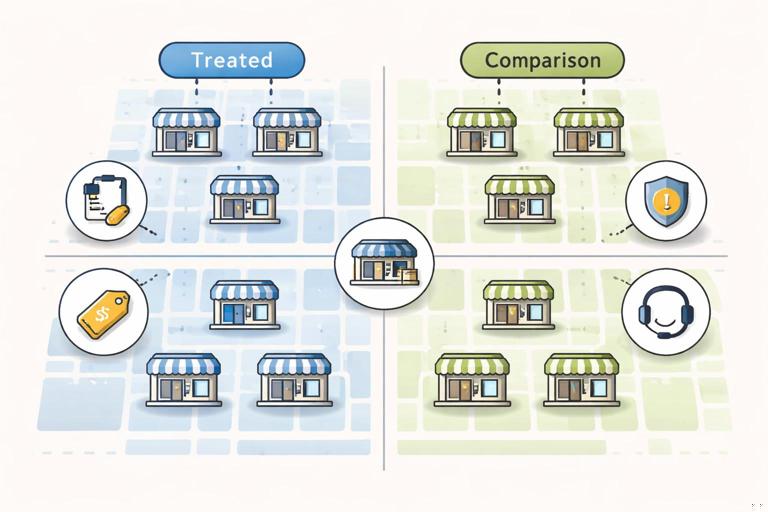
Difference-in-Differences (DiD) is a quasi-experimental method used to estimate the causal impact of a change when randomization is not feasible, but you have data before and after the change for a treated group and a comparison group. It is especially useful for business situations where a policy, pricing rule, or operational tweak is introduced in one region, store, channel, team, or time window, while other comparable units do not receive the change at the same time.

Typical business uses include: a new return policy rolled out in one set of stores, a pricing shift applied to a subset of markets, a new staffing model in certain warehouses, a fraud rule change for one payment method, or a new customer support workflow for one queue. In each case, you want to separate the effect of the change from other forces happening over time (seasonality, macro demand, competitor actions, platform changes).

DiD does this by comparing changes over time, not levels. The core idea is: if treated and comparison groups would have moved in parallel absent the change, then any extra change in the treated group after the intervention can be attributed to the intervention.

The Core Setup and the DiD Estimator

Notation and intuition

You observe an outcome (for example, revenue per store per day) for two groups across two periods: pre-change and post-change. One group is exposed to the change (treated), the other is not (control/comparison). DiD computes:

• Change in treated group: (Post − Pre) for treated
• Change in comparison group: (Post − Pre) for comparison
• Difference-in-differences: (Treated change) − (Comparison change)

This removes time-invariant differences between groups (e.g., treated stores are larger on average) and removes common time shocks (e.g., a holiday week increases demand everywhere). What remains is the incremental change that is specific to the treated group after the intervention.

Continue in our app.

• Listen to the audio with the screen off.
• Earn a certificate upon completion.
• Over 5000 courses for you to explore!

Or continue reading below...

Download the app

Two-by-two numeric example (policy change)

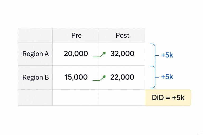
Suppose you change a return policy in Region A stores (treated) but not in Region B stores (comparison). Outcome is weekly net revenue per store.

• Region A (treated): Pre = $100k, Post = $112k (change = +$12k)
• Region B (comparison): Pre = $90k, Post = $97k (change = +$7k)

DiD estimate = $12k − $7k = +$5k per store per week. The interpretation is: after accounting for the overall upward trend seen in Region B, Region A increased an additional $5k that is attributed to the policy change.

Regression form (most common in practice)

With many units and many time periods, DiD is typically estimated with a regression that includes unit and time fixed effects. A standard specification is:

Y_it = α + β * Treat_i * Post_t + γ_i + δ_t + ε_it

Where:

• Y_it is the outcome for unit i at time t (store-day, market-week, warehouse-shift, etc.).
• Treat_i indicates treated units.
• Post_t indicates post-intervention periods.
• γ_i are unit fixed effects (control for stable differences across units).
• δ_t are time fixed effects (control for shocks common to all units at time t).
• β is the DiD estimate of the average treatment effect on the treated under the parallel trends assumption.

In many business settings you will add controls (e.g., weather, marketing spend, inventory availability) and sometimes allow different trends by group, but the key identifying variation is still the treated-vs-comparison divergence after the change.

The Key Assumption: Parallel Trends (and What It Really Means)

DiD relies on the idea that, absent the intervention, the treated group would have followed the same outcome trend as the comparison group. This does not require the groups to have the same level of the outcome, only the same trajectory over time in the absence of treatment.

In business terms, parallel trends is plausible when treated and comparison units are exposed to similar external forces and have similar underlying dynamics. It becomes less plausible when treated units are chosen precisely because they were already trending differently (for example, you apply a pricing shift only in markets where demand is accelerating, or you deploy an operational tweak only in warehouses with deteriorating performance).

How to assess parallel trends with pre-period data

You cannot directly observe the counterfactual trend post-change, but you can look for evidence in the pre-period:

• Visual check: Plot average outcome over time for treated and comparison groups. Look for similar slopes before the intervention.
• Placebo tests: Pretend the intervention happened earlier and estimate a “fake” DiD. You want near-zero effects in pre-periods.
• Event-study (dynamic DiD): Estimate effects at multiple leads/lags relative to the intervention date. Pre-treatment coefficients should be close to zero if trends are parallel.

These checks do not prove the assumption, but they can reveal obvious violations and help you choose a better comparison group or a better modeling approach.

Step-by-Step: Running a DiD for a Pricing Shift

Consider a pricing shift: you increase prices by 3% in a subset of markets due to cost changes, while other markets keep prices unchanged for now. You want the causal effect on contribution margin and units sold.

Step 1: Define the unit of analysis and time granularity

Choose a unit that matches how the pricing change is applied and how outcomes respond:

• Unit: market-SKU-week, market-category-week, or store-week.
• Time: weekly is often a good compromise for pricing (daily can be noisy; monthly may hide dynamics).

Ensure the intervention date is well-defined. If the change is phased in over several days, define the “effective” start date and consider excluding the transition week.

Step 2: Define treated and comparison groups

Treated markets are those where the price changed. Comparison markets should be as similar as possible and not affected by spillovers (e.g., customers crossing borders to buy cheaper). Practical tactics:

• Exclude markets adjacent to treated markets if cross-market substitution is likely.
• Match on pre-period levels and trends of key outcomes (units, revenue, margin) and on market characteristics (income, competition intensity, channel mix).
• Use multiple comparison markets rather than a single “best” market to reduce idiosyncratic noise.

Step 3: Choose outcomes and guardrails

For pricing, outcomes often include:

• Primary: contribution margin per market-week, profit, or gross margin dollars.
• Mechanism metrics: units sold, conversion rate, average order value.
• Guardrails: refund rate, customer complaints, churn, stockouts (to ensure you are not misattributing supply issues to price).

Make sure outcomes are measured consistently across markets and time. Pricing analyses are particularly sensitive to changes in product mix, promotions, and inventory availability.

Step 4: Build the panel dataset

Create a table with one row per unit-time (e.g., market-week) including:

• Outcome(s) Y
• Treat indicator (1 for treated markets)
• Post indicator (1 for weeks after the change)
• Time-varying controls: promo intensity, ad spend, competitor price index (if available), stockout rate, seasonality flags
• Identifiers for unit and time fixed effects

Include enough pre-period to assess trends (often 8–20 weeks depending on seasonality) and enough post-period to capture steady-state effects (but be careful if other changes occur later).

Step 5: Estimate the DiD regression with fixed effects

Y_it = α + β * Treat_i * Post_t + γ_i + δ_t + θ'X_it + ε_it

Where X_it are controls. Interpret β as the average incremental change in the outcome attributable to the pricing shift.

Step 6: Use correct uncertainty estimates (standard errors)

In DiD, errors are often correlated within units over time (a market has persistent shocks). Use clustered standard errors at the unit level (e.g., market). If treatment is assigned at a higher level (e.g., region), cluster at that level. If you have few clusters, consider methods designed for small numbers of clusters (for example, wild cluster bootstrap) to avoid overly optimistic confidence intervals.

Step 7: Validate with an event-study and robustness checks

Estimate dynamic effects to see whether the impact grows, decays, or appears before the intervention (a red flag). A common event-study specification is:

Y_it = α + Σ_k β_k * Treat_i * 1[t = k relative to intervention] + γ_i + δ_t + ε_it

Robustness checks that are often practical in pricing contexts:

• Exclude weeks with major promotions or holidays and see if results hold.
• Use alternative comparison sets (e.g., matched markets vs. all untreated markets).
• Check sensitivity to including inventory/stockout controls.
• Run the model on outcomes that should not move (placebo outcomes) to detect spurious effects.

Policy Changes: Handling Compliance, Eligibility, and Partial Exposure

Business “policy changes” often have messy exposure. Examples: a new free-shipping threshold, a revised refund window, or a change in eligibility rules for discounts. Not every customer in a treated region may be equally exposed (some never return items; some never hit the shipping threshold).

Intent-to-treat vs. treatment-on-the-treated in DiD language

If the policy is rolled out at the region/store level, DiD naturally estimates an intent-to-treat effect: the average impact of being in a region where the policy is in place, regardless of whether each individual “uses” it. This is often the right estimand for decision-making (what happens if we implement the policy in a region?).

If you need an effect among compliers (those who are actually affected), you may need additional structure (e.g., an instrument for exposure intensity) or a design that leverages eligibility cutoffs. In many operational settings, staying with intent-to-treat is more robust and aligns with rollout decisions.

Staggered adoption across regions

Policies are frequently rolled out in waves. This creates multiple treated cohorts with different start dates. A simple two-period DiD is no longer sufficient. You can still use DiD ideas, but you must use an estimator appropriate for staggered timing to avoid bias from using already-treated units as controls.

Practically, you can:

• Define cohorts by adoption date and estimate cohort-specific effects over event time (relative to each cohort’s start).
• Aggregate effects using modern DiD estimators designed for staggered adoption (cohort-time average treatment effects).

Even if you do not implement the full methodology immediately, you should at minimum avoid comparing late adopters (untreated yet) to early adopters (already treated) without accounting for treatment timing.

Operational Tweaks: Warehouses, Support Teams, and Process Changes

Operational changes often affect throughput, quality, and cost simultaneously. Examples: a new picking algorithm in a warehouse, a revised call routing rule in customer support, or a new QA checklist in manufacturing. DiD can work well because operations data is typically high-frequency and available for many comparable units.

Example: warehouse process change

You introduce a new packing workflow in 5 warehouses (treated) starting on a given week. You keep 10 similar warehouses unchanged (comparison). Outcomes include:

• Orders shipped per labor hour (productivity)
• Late shipment rate (service level)
• Damage rate (quality)
• Overtime hours (cost/strain)

A DiD analysis can estimate the net effect on each outcome, but operational settings require extra attention to interference and capacity constraints. If treated warehouses absorb overflow from untreated warehouses (or vice versa), the comparison group may be indirectly affected, weakening the design. In that case, consider redefining units (e.g., by network region) or explicitly modeling spillovers.

Step-by-step: operational DiD checklist

• Map exposure: confirm which units truly changed process and when; exclude transition days.
• Stability of measurement: verify that logging definitions did not change with the process (e.g., a new scanner changes timestamps).
• Capacity and routing: check whether work was reallocated across units after the change.
• Pre-trend diagnostics: plot outcomes for 4–12 weeks pre-change; look for divergence.
• Multiple outcomes: estimate productivity and quality jointly (at least report both) to avoid “improvement” that is actually cost shifting.
• Clustered uncertainty: cluster at warehouse level; if only a few warehouses, use small-cluster robust methods.

Common Failure Modes and How to Mitigate Them

1) Comparison group is contaminated (spillovers)

Pricing changes can cause customers to switch markets; policy changes can shift demand across channels; operational changes can reroute work. If the comparison group is affected, DiD underestimates or misstates the effect.

Mitigations:

• Choose comparison units with minimal interaction (geographic buffers, separate channels).
• Measure spillover indicators (cross-border traffic, rerouted volume) and run sensitivity analyses excluding high-spillover units.

2) Different underlying trends (non-parallel trends)

If treated units were already improving or deteriorating faster, DiD will attribute that difference to the intervention.

Mitigations:

• Use a better-matched comparison set based on pre-period trends.
• Add group-specific linear trends cautiously (useful when trends differ smoothly, risky when it overfits).
• Use an event-study to detect pre-trend differences and reconsider the design if leads are non-zero.

3) Other simultaneous changes (bundled interventions)

A pricing shift might coincide with a marketing campaign; a policy change might coincide with a website redesign; an operational tweak might coincide with staffing changes. DiD will capture the combined effect unless you can separate them.

Mitigations:

• Control for observable concurrent changes (promo spend, staffing levels).
• Restrict the analysis window to a period with fewer overlapping changes.
• Use multiple treated groups with different timings if available, to disentangle effects.

4) Anticipation effects

Teams or customers may react before the official start date (e.g., sales reps pre-emptively discount, customers stock up before a price increase). This can create apparent pre-treatment effects.

Mitigations:

• Use event-study leads to detect anticipation.
• Redefine the intervention start date to when behavior actually changed.
• Exclude a “ramp” period around the change.

5) Composition changes

After a pricing change, the mix of customers or products may shift. Your outcome might change because the population changed, not because behavior changed within the same population.

Mitigations:

• Analyze outcomes at a more granular level (SKU-market-week) and aggregate consistently.
• Track mix metrics (share of premium SKUs, new vs. returning customers).
• Consider reweighting to a fixed pre-period mix for a decomposition.

Extensions You Will Use in Real Business DiD

Multiple time periods and seasonality

Most business data has strong seasonality (day-of-week, month, holidays). Time fixed effects handle common seasonality if it affects treated and comparison similarly. If seasonality differs by group (e.g., coastal markets have different peaks), you may need interactions (group-by-season fixed effects) or a more tailored comparison set.

Continuous treatment intensity (not just on/off)

Some changes vary in intensity: a 1% to 5% price increase across markets, or different degrees of staffing changes. You can model intensity by replacing the binary interaction with a continuous measure:

Y_it = α + β * Intensity_it + γ_i + δ_t + ε_it

Where Intensity_it might be the percent price change (0 for untreated markets). Interpretation becomes “effect per unit of intensity.” Ensure intensity is not chosen in response to expected outcomes (which would reintroduce bias).

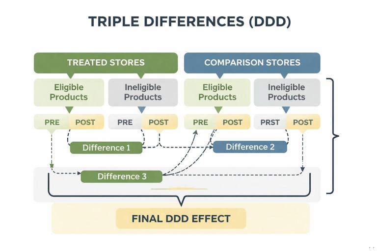
Triple differences (Difference-in-Difference-in-Differences)

Sometimes you can add a third dimension to strengthen identification. Example: a policy change affects only a subset of products (eligible SKUs) within treated stores. You can compare eligible vs. ineligible products across treated vs. comparison stores over time. This can help control for store-level shocks and time shocks more tightly.

A stylized setup:

• Dimension 1: treated vs. comparison stores
• Dimension 2: eligible vs. ineligible products
• Dimension 3: pre vs. post

The triple-difference estimate isolates the incremental change for eligible products in treated stores after the policy, netting out broader store and product trends.

Implementation Notes: Data, Modeling Choices, and Reporting

Choosing the right aggregation

DiD can be run at customer level, transaction level, store-day, or market-week. Choose the level that reflects how treatment is assigned and how interference might occur. For pricing and policy changes, market-week or store-week is often stable and interpretable. For operational changes, shift-level or day-level may capture immediate effects but can be noisy.

Reporting results in business terms

Translate β into decision-relevant units:

• Incremental margin dollars per market-week and total impact over the rollout footprint
• Incremental units and implied price elasticity (if you also track price changes)
• Operational savings (labor hours) and service-level changes (late rate)

Always report uncertainty (confidence intervals) and show the pre/post trends plot. For stakeholders, the trend plot often communicates validity better than the regression table.

Minimum set of artifacts to produce

• Definition of treated/comparison units and intervention timing
• Pre-trend plots and event-study coefficients
• Main DiD estimate with clustered standard errors
• At least two robustness checks (alternative comparison set, alternative window, placebo)
• Impact translation (per-unit and total) for primary outcome and guardrails