Counterfactuals, Confounders, and Selection Bias in Real Decisions

Why real decisions need counterfactual thinking

In business, you rarely get to observe what would have happened if you had chosen differently. You launch a discount, but you cannot simultaneously see the same customers in the same week without the discount. You hire a sales rep, but you cannot observe the same territory in the same quarter without that rep. This missing “what if” outcome is the counterfactual. Causal inference is largely the discipline of making careful, defensible statements about counterfactuals using the data you do have.

A useful way to frame it is: for each unit (a customer, store, employee, session), there are multiple potential outcomes—one for each action you could take. You only observe one of them, the one corresponding to the action actually taken. The gap between observed outcomes and unobserved potential outcomes is why naive comparisons often mislead.

Potential outcomes in plain business language

Suppose you are deciding whether to offer free shipping (treatment) to a customer. For each customer i there are two potential outcomes: Y_i(1) = whether they purchase if offered free shipping, and Y_i(0) = whether they purchase if not offered free shipping. You observe only one: if they were offered free shipping, you observe Y_i(1); otherwise you observe Y_i(0). The individual causal effect is Y_i(1) − Y_i(0), but it is never fully observed for any single person.

Because individual effects are unobservable, decision-making typically targets average effects such as the Average Treatment Effect (ATE): E[Y(1) − Y(0)], or the effect for a relevant segment (e.g., new customers, high-intent visitors, churn-risk accounts). The core challenge is to estimate these averages without confusing cause with correlation.

Confounders: the hidden reasons groups differ

A confounder is a variable that influences both the action taken (treatment assignment) and the outcome. Confounders create spurious associations: the treated group looks different from the untreated group even before the treatment happens, so differences in outcomes cannot be attributed to the treatment alone.

Continue in our app.

• Listen to the audio with the screen off.
• Earn a certificate upon completion.
• Over 5000 courses for you to explore!

Or continue reading below...

Download the app

Concrete example: “VIP outreach” and revenue

Imagine a sales team runs VIP outreach calls to accounts that appear most likely to buy. After a quarter, accounts that received VIP outreach have higher revenue than those that did not. It is tempting to say the outreach caused the revenue lift. But the outreach was targeted: high-propensity accounts were more likely to be called and also more likely to buy regardless of outreach. “Propensity to buy” (or its proxies like past spend, engagement, lead score) is a confounder.

• Treatment: received VIP outreach call
• Outcome: quarterly revenue
• Confounders: past spend, lead score, pipeline stage, account size, seasonality, product fit

If you compare treated vs untreated without adjusting for these confounders, you will overestimate the effect of outreach (because the treated group was “better” to begin with).

How confounding shows up in real data

Confounding often appears as systematic baseline differences:

• Treated customers have higher prior purchase frequency.
• Stores that adopt a new process earlier are in higher-income neighborhoods.
• Employees selected for training are top performers.
• Users who see a feature are those who updated the app (and are more engaged).

A practical diagnostic is to compare pre-treatment variables between groups. If the treated group differs materially on variables that predict the outcome, you should assume confounding is present unless assignment was randomized.

Selection bias: when your sample is not the population you think it is

Selection bias occurs when the data you analyze are selected in a way that depends on variables related to the outcome, the treatment, or both. The result is that your estimate applies to a distorted subset, or is biased even for that subset. Selection bias is not just “non-representative sampling” in a marketing sense; it can be created by product flows, eligibility rules, missing data, and post-treatment filtering.

Common business forms of selection bias

• Survivorship bias: analyzing only customers who remained active, ignoring those who churned earlier.
• Eligibility/targeting filters: evaluating a program only among those who met a threshold (e.g., “only users with 3+ sessions”), where the threshold is affected by the treatment.
• Opt-in bias: users who choose to enroll in a program differ from those who do not (motivation, time, need).
• Missingness bias: outcomes are missing more often for certain groups (e.g., NPS surveys answered mainly by very happy or very unhappy customers).

Example: measuring the impact of a retention email

You send a retention email to users predicted to churn. You then measure churn among users who opened the email versus those who did not. This is a classic selection trap: “open” is not randomly assigned. Openers are typically more engaged and less likely to churn anyway. The act of conditioning on opening creates selection bias because opening is influenced by both user engagement and the email itself, and engagement also influences churn.

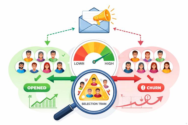
Better comparisons would be: (1) randomized assignment to receive the email or not, regardless of opening; or (2) observational methods that adjust for confounders affecting assignment, without conditioning on post-treatment variables like opens.

Counterfactuals meet confounders and selection: a mental model with causal graphs

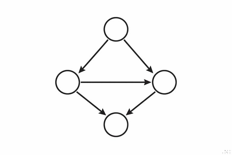
A practical way to reason about confounding and selection is to draw a simple causal diagram (a directed acyclic graph, DAG). You do not need advanced graph theory; you need a disciplined habit of stating what causes what.

Confounding pattern

Confounding is typically: Z → T and Z → Y, where Z is a confounder, T is treatment, Y is outcome. If you ignore Z, the association between T and Y mixes causal effect with baseline differences.

Z (confounder) --> T (treatment) --> Y (outcome)  (causal path)  Z (confounder) --> Y (outcome)  (backdoor path)

To estimate the causal effect of T on Y, you aim to “block” the backdoor path through Z by adjusting for Z (e.g., stratification, regression, matching, weighting), assuming Z is measured and correctly modeled.

Selection/collider pattern

Selection bias often arises when you condition on a variable S that is influenced by both T and Y (or their causes). S is a collider: T → S ← Y. Conditioning on S opens a spurious association between T and Y even if none exists causally.

T (treatment) --> S (selected/observed) <-- Y (outcome)  Condition on S => induces correlation between T and Y

In business terms, “only analyze users who returned next week” is conditioning on a post-treatment variable that is related to the outcome. This can create misleading results, often reversing the apparent direction of effects.

Step-by-step: how to identify confounders and selection bias before you model

Step 1: Define the decision, treatment, and outcome precisely

Ambiguity creates hidden bias. Write down:

• Unit: customer, account, store, session, employee?
• Treatment: what exactly changes? (e.g., “discount of 10% offered at checkout”)
• Outcome: what metric and time window? (e.g., “purchase within 7 days”)
• Timing: when is treatment assigned relative to outcome measurement?

Timing is crucial: confounders must be pre-treatment. Variables measured after treatment may be mediators (part of the causal pathway) or colliders (selection variables), and adjusting for them can bias estimates.

Step 2: List plausible causes of treatment assignment

Ask: “Why did some units receive the treatment and others not?” In real operations, assignment is rarely random. Common drivers include:

• Rules (eligibility thresholds, routing logic)
• Human judgment (sales prioritization, manager discretion)
• Customer behavior (self-selection, opt-in)
• System constraints (inventory, staffing, budget caps)

Each driver is a candidate confounder if it also affects the outcome.

Step 3: List plausible causes of the outcome

Ask: “What else moves this metric?” For revenue, think demand, seasonality, pricing, competitor actions, product availability, macro conditions, customer lifecycle stage. For churn, think product usage, support experience, contract terms, onboarding quality.

Step 4: Identify overlap: variables that cause both assignment and outcome

The intersection of Steps 2 and 3 is your confounder set. Examples:

• Lead score affects outreach assignment and purchase probability.
• Prior engagement affects feature exposure and retention.
• Store foot traffic affects adoption of staffing changes and sales.

Then check whether these variables are measured before treatment. If not, you may need proxies, alternative designs, or to accept that the effect is not identifiable from available data.

Step 5: Identify selection mechanisms in your dataset

Ask: “Who is missing, and why?” and “What filters did we apply?” Common selection points:

• Only users who logged in (excludes churned or inactive)
• Only customers who reached checkout (excludes earlier funnel stages)
• Only tickets with a satisfaction response (nonresponse bias)
• Only accounts with complete CRM fields (missingness correlated with rep behavior)

Write down the selection variable explicitly (e.g., “has outcome recorded,” “reached stage X,” “responded to survey”). Then ask whether selection is influenced by treatment, outcome, or their causes.

Step 6: Draw a minimal DAG and decide what to adjust for

Keep it minimal: include treatment, outcome, key confounders, and any selection variables you might condition on. Use the DAG to decide:

• Adjust for: pre-treatment confounders that open backdoor paths.
• Do not adjust for: mediators (post-treatment variables on the causal path) if you want total effect.
• Avoid conditioning on: colliders and selection variables that can open spurious paths.

This step prevents common mistakes like controlling for “email opens” or “post-treatment engagement” when estimating the effect of sending the email.

Practical patterns and how to handle them

Pattern 1: Targeted interventions (propensity-driven assignment)

Scenario: A churn-prevention offer is given to customers with high churn risk.

Risk: Confounding by risk score and its components (usage decline, complaints, payment issues).

Practical handling:

• Ensure all variables used in targeting are captured as pre-treatment covariates.
• Estimate effects within strata of risk (e.g., deciles) to compare like with like.
• Use weighting or matching to balance covariates between treated and untreated.

Operational check: If the model says the offer “increases churn,” verify whether the treated group had much higher baseline risk. This is often a sign of residual confounding or poor overlap (treated units have no comparable controls).

Pattern 2: Feature exposure depends on user behavior

Scenario: A new in-app tutorial appears after a user completes onboarding step 3. You compare retention of users who saw the tutorial vs those who did not.

Risk: Selection bias and confounding: users who reach step 3 are more engaged and more likely to retain. “Reached step 3” is a gate that selects a non-random subset.

Practical handling:

• Redefine the unit and estimand: effect of tutorial among users who reached step 3 (explicitly conditional), or effect of changing the onboarding flow earlier.
• If possible, randomize tutorial display among users who reach step 3 (clean within-gate experiment).
• Avoid comparing “saw tutorial” vs “did not” across the whole user base without accounting for the gate.

Pattern 3: Conditioning on post-treatment outcomes (“only converters”)

Scenario: You test two landing pages and analyze average order value only among users who purchased.

Risk: Selection bias: purchase is affected by the landing page and also related to order value. Conditioning on purchasers can distort the comparison (you are comparing different mixes of buyers).

Practical handling:

• Prefer metrics defined for all assigned users (e.g., revenue per visitor, conversion rate, expected value).
• If you must analyze among purchasers, treat it as a different estimand and be explicit: “effect on AOV among purchasers,” not “effect on revenue.”
• Use methods designed for principal strata only with strong assumptions; otherwise avoid over-interpreting.

Pattern 4: Survey outcomes and nonresponse

Scenario: You change support scripts and measure impact on CSAT, but only 15% respond.

Risk: Selection bias if response depends on satisfaction, time, issue severity, or treatment (e.g., new script encourages responses).

Practical handling:

• Track response rate as an outcome itself; changes in response rate are informative.
• Model response propensity using pre-treatment variables (issue type, channel, customer tier) and use inverse probability weighting to reweight respondents.
• Where feasible, collect outcomes passively (repeat contact, churn) to triangulate.

Step-by-step: a practical workflow to reduce bias in observational decision analysis

Step 1: Create a “pre-treatment snapshot” table

For each unit, build features measured strictly before treatment assignment: prior behavior, demographics/firmographics, historical outcomes, seasonality indicators, channel, geography. Freeze the snapshot at a clear cutoff time.

This prevents leakage of post-treatment information into your adjustment set, which can silently introduce bias.

Step 2: Check overlap and positivity

Even with confounders measured, you need overlap: for each covariate profile, there should be both treated and untreated units. If a segment is always treated (or never treated), you cannot learn the counterfactual from data.

• Inspect treatment rates by key segments (risk decile, region, tier).
• Plot propensity score distributions for treated vs untreated; limited overlap signals extrapolation risk.

Step 3: Balance diagnostics before trusting effect estimates

After matching/weighting/adjustment, check whether treated and control groups are similar on pre-treatment covariates.

• Compare standardized mean differences for key covariates.
• Check balance within important segments (not just overall).

If balance is poor, your estimate is likely still confounded, regardless of how sophisticated the model is.

Step 4: Avoid conditioning on mediators and colliders

Make a “do-not-control” list of post-treatment variables such as:

• Opens/clicks after an email is sent
• Usage after a feature is enabled
• Intermediate funnel steps after a landing page change
• Any variable that could be affected by the treatment

If you include these in a regression “because they predict the outcome,” you may be estimating a different causal quantity (direct effect) or introducing selection bias.

Step 5: Sensitivity thinking for unmeasured confounding

In many real settings, some confounders are unobserved (e.g., motivation, competitor outreach, informal discounts). You should explicitly ask how strong an unmeasured confounder would need to be to explain away the observed effect.

Practically:

• Compare effect estimates across multiple adjustment sets (minimal vs rich) to see stability.
• Use negative control outcomes (metrics that should not be affected) to detect residual bias.
• Use negative control exposures (placebo treatments) when available.

These checks do not “prove” causality, but they help prevent confident decisions based on fragile estimates.

Worked example: pricing change with confounding and selection traps

Decision: Increase price by 5% for a subset of customers.

Naive analysis: Compare churn for customers who experienced the price increase vs those who did not.

Where it goes wrong:

• Confounding: Price increases may be applied to customers out of contract, on certain plans, or in certain regions—factors that also affect churn.
• Selection bias: If you analyze only customers who renewed (because churned customers have incomplete billing records), you condition on a post-treatment outcome-related selection.

Step-by-step correction approach:

• 1) Define timing: treatment assignment date = date price increase is communicated; outcome window = churn within 90 days after that date.
• 2) Pre-treatment covariates: tenure, plan type, prior discounts, usage trend, support tickets, region, contract status, renewal date proximity.
• 3) Ensure complete outcome capture: build churn from account status logs rather than billing records to avoid missing churned customers.
• 4) Adjust for confounders: compare treated vs untreated within contract-status strata; use weighting/matching on the snapshot covariates.
• 5) Check overlap: if all out-of-contract customers were treated, you cannot estimate the effect for that group without additional design (e.g., phased rollout).

This example illustrates a general rule: many “data availability” shortcuts are actually selection mechanisms that bias the estimate.

Practical checklist: what to ask in stakeholder reviews

• Counterfactual clarity: What is the alternative action we are comparing against, and is it realistic?
• Assignment logic: Who got the treatment and why? Was any part random?
• Pre-treatment snapshot: Are all adjustment variables measured before treatment?
• Selection filters: Did we exclude anyone based on post-treatment behavior (converters, responders, actives)?
• Overlap: Do we have comparable untreated units for treated units (and vice versa)?
• Outcome measurement: Is the outcome observed for everyone, or only a selected subset?
• Robustness: Do results hold across reasonable alternative specifications and segments?