Why causal diagrams (DAGs) matter for identification
When you want to estimate a causal effect (for example, the effect of a marketing campaign on revenue), the hardest part is often not modeling or prediction; it is deciding whether the effect is identifiable from the data you can collect. Directed acyclic graphs (DAGs) are a practical tool to make identification decisions explicit. A DAG is a diagram of variables connected by arrows that represent direct causal influence, with the constraint that you cannot follow arrows and return to the same variable (no cycles). The DAG is not “the data”; it is a structured statement of assumptions about how the world works. Identification is the process of translating those assumptions into a valid adjustment strategy: which variables to control for, which to avoid, and what causal quantity is recoverable from observed data.
In business settings, teams often jump from “we have a dataset” to “let’s run a regression controlling for everything.” DAGs help prevent that reflex by forcing a disciplined question: which paths create spurious association between treatment and outcome, and which variables would block those paths without introducing new bias?
Core elements of a DAG
Nodes, arrows, and acyclicity
Each node is a variable (measured or unmeasured). An arrow X → Y means X is a direct cause of Y, given the other variables in the graph. “Direct” does not mean “immediate in time”; it means there is no other measured variable in the graph that fully mediates that causal influence. Acyclic means you cannot have feedback loops like A → B → A. In practice, many business systems have feedback (e.g., pricing affects demand, demand affects pricing). For DAG-based identification, you typically represent a single decision point or a time-sliced snapshot (e.g., price at week t affects demand at week t, and demand at week t affects price at week t+1). Time indexing is a common way to keep the graph acyclic.
Parents, children, ancestors, descendants
For a node X, its parents are nodes with arrows into X; its children are nodes with arrows out of X. Ancestors are parents of parents (and so on), and descendants are children of children. These relationships matter because many identification rules refer to “descendants of treatment” or “ancestors of outcome.”
Paths and what it means to “block” them
A path is any sequence of connected edges (ignoring arrow direction). Causal identification often hinges on whether certain paths between treatment (T) and outcome (Y) are open (transmit association) or blocked (do not transmit association) after conditioning on a set of variables Z. The key concept is d-separation, which provides a graphical criterion for when a set Z blocks all non-causal paths between T and Y.
- Listen to the audio with the screen off.
- Earn a certificate upon completion.
- Over 5000 courses for you to explore!

Download the app
d-separation in practice: chains, forks, and colliders
Most DAG reasoning reduces to three local patterns. Understanding them is enough to apply the backdoor criterion correctly.
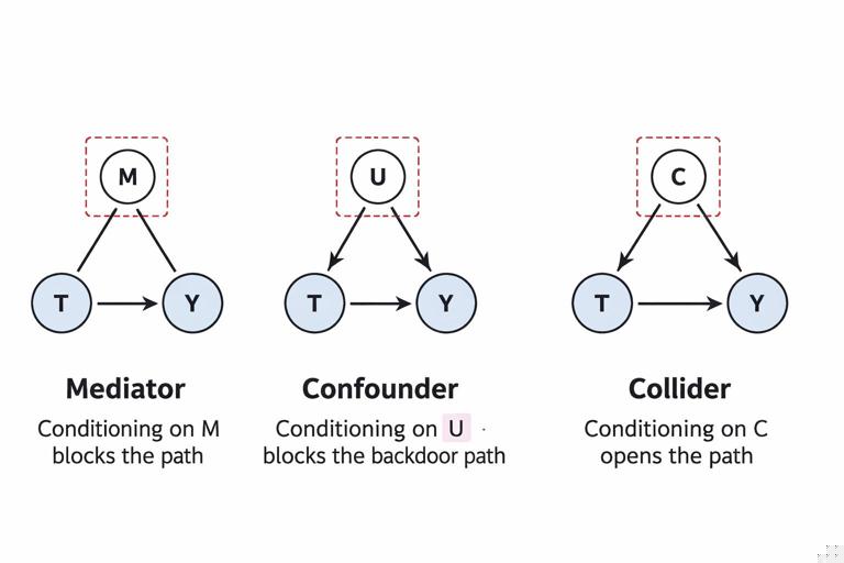
Chain (mediator pattern): T → M → Y
M lies on a causal chain from T to Y. If you condition on M, you block the path from T to Y through M. That is useful if you want the direct effect of T on Y not mediated by M, but it is harmful if you want the total effect of T on Y. In business terms: if T is “discount offer,” M is “purchase probability,” and Y is “revenue,” conditioning on purchase probability would remove part of the effect you’re trying to measure.
Fork (common cause pattern): U → T and U → Y
U is a common cause of T and Y. This creates a non-causal (backdoor) path T ← U → Y that induces association even if T has no causal effect on Y. Conditioning on U blocks this path and is typically what people mean by “adjusting for confounding.”
Collider: T → C ← Y (or T ← U1 → C ← U2 → Y)
A collider is a node with two arrows pointing into it. Colliders are special: the path through a collider is blocked by default. Conditioning on a collider (or on its descendants) opens the path and can create spurious association. This is the main reason “control for everything” can backfire. A common business example: T is “ad exposure,” Y is “purchase,” and C is “website visit.” If both ad exposure and purchase propensity influence the likelihood of visiting the website, conditioning on website visit can induce a false relationship between ad exposure and purchase even if none exists (or distort the true effect).
Identification target: total effect vs direct effect
Before applying any criterion, you must define the estimand: what causal effect do you want? The total effect of T on Y includes all causal pathways from T to Y. A controlled direct effect or natural direct effect aims to isolate the effect not mediated by certain variables. DAGs help you see which variables are mediators and which are confounders. The backdoor criterion is primarily used to identify the total effect by blocking non-causal paths without blocking causal paths.
The backdoor criterion: what it is and why it works
The backdoor criterion provides a sufficient condition for identifying the causal effect of T on Y from observational data by adjusting for a set of variables Z. Intuitively, you want to block every path from T to Y that starts with an arrow into T (a “backdoor” path), because those paths represent non-causal association. At the same time, you must not condition on variables that would introduce bias (notably colliders) or block the causal effect you want (mediators, if estimating total effect).
Formal statement (graphical)
A set of variables Z satisfies the backdoor criterion relative to (T, Y) if:
- No variable in Z is a descendant of T.
- Z blocks every path between T and Y that contains an arrow into T.
If such a set Z exists and all variables in Z are measured, then the total causal effect is identifiable by adjustment:
P(Y | do(T=t)) = Σ_z P(Y | T=t, Z=z) P(Z=z)In estimation terms, you can use regression, matching, weighting, or stratification to estimate the conditional outcome model P(Y | T, Z) and then average over the distribution of Z.
Step-by-step workflow: using a DAG to choose an adjustment set
Step 1: Define treatment, outcome, and time window
Pick a specific intervention and outcome with a clear time ordering. Example: T = “received retention email in week 0,” Y = “renewed subscription by week 4.” Time anchoring helps avoid accidental cycles and clarifies what can be a descendant of T.
Step 2: List candidate variables and draft causal relationships
Brainstorm variables that plausibly affect T and/or Y: customer tenure, prior engagement, plan type, region, support tickets, prior churn risk score, etc. Then draw arrows reflecting your best causal assumptions. The goal is not to include every variable in the company database; it is to include the variables that matter for causal pathways between T and Y and for selection into T.
Step 3: Identify backdoor paths from T to Y
Trace all paths between T and Y that begin with an arrow into T. These are the paths that can create spurious association. For each path, determine whether it is open or blocked by default (colliders block by default; chains and forks are open by default).
Step 4: Propose Z sets that block all backdoor paths without conditioning on descendants of T
Choose variables that block each open backdoor path. Prefer variables that are common causes (fork blockers) rather than mediators. Avoid colliders and descendants of colliders unless you are sure you need them and understand the consequences.
Step 5: Check for “bad controls”
Verify that none of the chosen Z variables are: (a) descendants of T, (b) colliders on any relevant path, or (c) variables that would open a collider path when conditioned on. This step is where many adjustment mistakes are caught.
Step 6: Translate the adjustment set into an estimation plan
Once Z is selected, decide how to estimate. For example, use inverse probability weighting with a propensity model P(T | Z) if you want a design-like approach, or use outcome regression E[Y | T, Z] if you want a modeling approach. The DAG tells you what to condition on; it does not dictate the estimator.
Practical example 1: Marketing campaign with a collider trap
Scenario: You want the effect of a paid social campaign (T) on purchases (Y). You have data on site visits (V), prior brand affinity (A), and retargeting eligibility (R). Consider the following causal story:
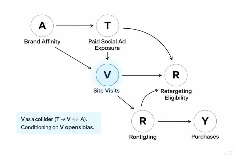
- A → T (people with higher affinity are more likely to be targeted or to engage with ads)
- A → Y (affinity increases purchase likelihood)
- T → V (ads drive visits)
- A → V (affinity also drives visits)
- V → R (visits make you eligible for retargeting lists)
- R → T (retargeting increases ad exposure)
- R → Y (retargeting can also increase purchases)
Key insight: V is a collider on T → V ← A. By default, that path is blocked. If you condition on V (e.g., analyze only visitors or include visits as a control), you open a non-causal path between T and A, and since A affects Y, you create bias. Additionally, conditioning on R can be tricky because R is downstream of V and also affects both T and Y, creating complex paths.
Backdoor paths into T include T ← A → Y and T ← R → Y (since R → T). To block T ← A → Y, adjust for A (brand affinity) if measured. To address T ← R → Y, you might adjust for R, but only if doing so does not open other collider paths. Because R is affected by V, and V is affected by T, R can be a descendant of T through T → V → R, violating the backdoor rule (no descendants of T). In this story, R is a post-treatment variable for some units, so adjusting for it can bias the total effect.
A safer adjustment set might be Z = {A} only, paired with a design that defines T as the initial campaign assignment before retargeting kicks in, or by redefining the treatment to include the whole ad exposure policy (initial + retargeting). The DAG forces you to confront that “retargeting eligibility” is not a harmless control; it is part of the treatment mechanism over time.
Practical example 2: Pricing change and seasonality as a backdoor path
Scenario: Estimate the effect of a price increase (T) on weekly sales (Y). Suppose:
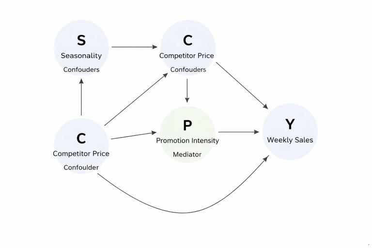
- S (seasonality) → T (prices are raised during peak season)
- S → Y (peak season increases sales)
- C (competitor price) → T (you respond to competitor moves)
- C → Y (competitor price affects your demand)
- T → P (promotion intensity changes after price change)
- P → Y
Backdoor paths include T ← S → Y and T ← C → Y. Adjusting for S and C blocks these. Promotion intensity P is a mediator (T → P → Y). If you adjust for P while trying to estimate the total effect of price on sales, you will remove the portion of the effect that operates through promotions. The DAG clarifies that P is not a confounder; it is part of the causal response to pricing.
An adjustment set Z = {S, C} satisfies backdoor (assuming neither is a descendant of T). Then you can estimate:
E[Y | do(T=t)] = Σ_{s,c} E[Y | T=t, S=s, C=c] P(S=s, C=c)In practice, S might be represented by week-of-year indicators, holiday flags, or demand index; C might be competitor price scraped weekly.
How to find adjustment sets systematically
Minimal vs sufficient adjustment sets
There can be many valid adjustment sets. A minimal adjustment set blocks all backdoor paths with as few variables as possible. Minimal sets are often preferred because they reduce variance and reduce the risk of measurement error and missingness. However, “minimal” is not always “best” if the minimal set includes variables that are hard to measure well; a slightly larger set with more reliable proxies can be more practical.
Using the DAG to avoid overcontrol
Common overcontrol patterns include:
- Adjusting for mediators when estimating total effects.
- Adjusting for colliders like “selected into analysis sample,” “opened the app,” “responded to survey,” or “qualified lead,” when those are influenced by both treatment and outcome drivers.
- Adjusting for post-treatment variables that are affected by the treatment, even if they also predict the outcome.
A useful habit is to label each candidate control as one of: pre-treatment common cause, mediator, collider, or descendant of a collider. Only the first category is typically safe for backdoor adjustment.
Unobserved variables and what DAGs can still tell you
DAGs can include unobserved nodes (often drawn as latent variables). If a backdoor path runs through an unobserved common cause U of T and Y, you cannot block it by conditioning unless you have a measured proxy that truly blocks the path (which requires strong assumptions). The DAG helps you diagnose when identification is impossible with simple adjustment and when you need a different strategy (for example, an instrumental variable, a front-door approach, a randomized experiment, or collecting new data). Even without introducing those alternative methods in detail, the key operational value is: the DAG makes the “why” of non-identification explicit, so you can decide whether to redesign the decision process or measurement plan.
Backdoor criterion checklist for business analyses
Checklist
- Is every variable you plan to adjust for measured before the treatment decision point?
- Have you listed every plausible common cause of treatment and outcome? If not, which ones are unmeasured?
- Did you accidentally condition on a variable that is caused by the treatment (post-treatment KPI, intermediate metric, downstream eligibility flag)?
- Did you condition on a collider (a variable influenced by two causes on the path), such as “engaged users,” “approved customers,” “responders,” or “visitors”?
- After choosing Z, can you trace every backdoor path and confirm it is blocked?
Common adjustment sets in typical company problems
These are patterns you can map into your own DAGs:
Product change (T) → retention (Y): adjust for pre-change user maturity, prior engagement, plan type, acquisition channel, and seasonality; avoid post-change engagement metrics.
Sales outreach (T) → conversion (Y): adjust for lead quality and prior intent signals; avoid conditioning on “scheduled a demo” if it is influenced by outreach and by latent intent.
Fraud model intervention (T) → chargebacks (Y): adjust for pre-intervention risk signals and merchant category; avoid conditioning on “manual review outcome” if it is influenced by both the model and investigator judgment correlated with fraud risk.
From DAG to estimation: a concrete adjustment recipe
Once you have a valid backdoor set Z, you can implement adjustment with a repeatable recipe. The DAG ensures the recipe targets the right estimand.
Recipe: g-formula (standardization) with a backdoor set
- Fit an outcome model for Y using T and Z (for example, linear regression for continuous Y, logistic regression for binary Y, or flexible ML with cross-fitting).
- For each unit i, predict two potential outcomes: Ŷ_i(t=1) and Ŷ_i(t=0) by setting T accordingly while keeping Z at observed values.
- Average predictions over the sample to estimate E[Y | do(T=1)] and E[Y | do(T=0)].
- Compute the effect as the difference (or ratio) between these averages.
In code-like pseudocode:
fit model: Y ~ T + Z  (or ML model with features [T, Z])
for each i:
  y1_i = predict(Y | T=1, Z=z_i)
  y0_i = predict(Y | T=0, Z=z_i)
ATE = mean(y1_i - y0_i)
The critical point is that Z comes from the DAG, not from automated feature selection. You can use flexible modeling, but the identification logic must remain grounded in the causal diagram.
Common pitfalls when drawing DAGs for real organizations
Mixing definitions of treatment
Teams often conflate “assigned to campaign,” “saw the campaign,” and “clicked the campaign.” These are different treatments with different DAGs. If you use “clicked” as T, then many variables (like interest) become causes of T and Y, and click becomes a post-exposure behavior. A clean DAG starts with a treatment definition that corresponds to an actionable intervention (e.g., assignment or eligibility) and a time point.
Forgetting measurement processes
Some nodes represent measurement rather than underlying constructs (e.g., “recorded revenue,” “tracked sessions”). Measurement can introduce selection or missingness mechanisms that behave like colliders. If tracking is affected by both treatment and user type, conditioning on “has tracking data” can open biasing paths. Including measurement nodes in the DAG can clarify whether your analysis sample is selected in a problematic way.
Leaving out policy and operational constraints
Treatment assignment in businesses is rarely random. It is driven by rules (eligibility thresholds, budgets, caps, sales prioritization). Those rules create arrows into T from operational variables. If you omit them, you may miss backdoor paths. For example, “sales capacity” might influence who gets outreach (T) and also correlate with quarter-end discounting that affects conversion (Y).
How to communicate DAG-based identification to stakeholders
DAGs are most useful when they become a shared artifact across data science, product, marketing, and operations. A practical way to present them is:
- Start with the treatment and outcome and draw only the most important nodes first.
- For each arrow, state the business rationale in one sentence (“prior engagement affects likelihood of receiving the email because the targeting rule uses engagement score”).
- Explicitly mark which nodes are measured and which are not.
- Show which variables you will adjust for and which you will not, with a short reason (“do not adjust for post-treatment engagement because it is a mediator”).
This turns “we controlled for X” into “we adjusted for X because it blocks this specific backdoor path,” making the analysis easier to audit and less dependent on individual intuition.